RUSSIAN JOURNAL OF EARTH SCIENCES, VOL. 20, ES3005, doi:10.2205/2020ES000700, 2020

Tracking the formation of the gradient part of the southeastern Baltic Sea cold intermediate layer

N. Stepanova^1,2, A. Mizyuk³

¹Shirshov Institute of Oceanology RAS, Moscow, Russia

²Institute of Physics and Technology, Dolgoprudny, Moscow region, Russia

³Marine Hydrophysical Institute RAS, Sevastopol, Russia

Abstract

[1] In order to study the peculiarities of the thermohaline structure of the Baltic Sea, we conducted a research based on the Copernicus Marine Environment Monitoring service (https://marine.copernicus.eu/) products and field data collected in 2004–2006. The study of the reanalysed Baltic Sea hydrography allows us to show that it adequately reproduces elements of the thermohaline structure of the cold intermediate layer obtained from the measurement data. Here we examine the hypothesis about the formation of a lower part of the cold intermediate layer in early spring under the influence of a mechanism related to the estuary salinity/density gradient along the main axis of the Baltic Sea. Several numerical experiments were carried out to analyse the back trajectories of Lagrangian particles in the southeastern Baltic Sea. The analysis showed that in the Gdask Basin, at the depth corresponding to the lower part of the cold intermediate layer, there are particles coming from the Bornholm Basin and the S{upsk Channel. This confirms the contribution of the estuary salinity gradient to the formation of the lower part of the cold intermediate layer.

1. Introduction

Intermediate and cold intermediate layers of the majority of large basins are usually formed due to advection mechanism. They are particularly dynamic in the inland seas, which have vertical salinity stratification and a sharp pycnocline due to the connection with the ocean.

Figure 1

A number of papers are devoted to investigations of the generation mechanisms, regions and times of colder water formation, time rates of its generation, volumes and thermohaline characteristics, as well as routes of circulation in a basin. The most detailed works were published on the Mediterranen Sea [Lascaratos et al., 1999; Menna and Poulain, 2010] and the Black Sea [Korotaev et al., 2014; Oguz and Besiktepe, 1999; Staneva and Stanev, 1997; Stanev and Staneva, 2001; Stanev et al., 2003]. With such a background, investigations of the Cold Intermediate Layer (CIL) of the Baltic Sea look very fragmentary and sparse. However, its complicated internal structure (Figure 1) is presented in recent publications [Stepanova, 2017; Stepanova et al., 2015], indicating significant contribution of advection to its formation. Study of the hydrological parameters of the deep part of the Baltic Sea complement existing knowledge of the bottom waters [Krechik et al., 2019], coastal zone [Kapustina et al., 2017]. They are also practically useful for studies such as Ponomarenko and Krechik [2018] that speak about interrelations between the distribution of the hydrological/hydrochemical parameters and the micropalaeontological data.

The CIL in the Baltic Sea is a layer of water located below the seasonal thermocline and above the bottom waters of Atlantic origin. It is manifested in the warm season in the vertical cross-sections or profiles of sea water temperature (Figure 1). The process of the CIL formation takes place during the spring period while water temperature in the upper layer the open sea increases [Hydrometeoizdat, 1992]. In summer its volume is about 1/3 of the Baltic Proper. It is shown in [Stepanova et al., 2015] that the CIL is presented in the southeastern part of the Baltic Sea during about 8 months of the year (from April to November).

Here we define the boundaries of the CIL as maximum of absolute value of water vertical temperature gradient, as in earlier papers [Stepanova, 2017; Stepanova et al., 2015], (Figure 1). It is shown that the CIL allocated by the proposed method has a clear structure in the southeastern part of the Baltic Sea [Stepanova, 2017]: quasi-homogeneous and salinity gradient sublayers are present on all profiles within the CIL (Figure 1).

The idea of forming the quasi-homogeneous salinity sublayer has been described in [Chubarenko and Stepanova, 2018; Stepanova, 2017]. The study indicates the formation of this sublayer by mechanisms associated with the wind action and differential coastal heating within separate basins of the sea.

The annual formation of the salinity gradient sublayer of the CIL (Figure 1) is considered in this paper. It occurs at the lower part of the CIL. Near-bottom waters of the Atlantic origin are located below it. A hypothesis is proposed explaining how the cold sublayer with the salinity increasing with depth ("the salinity gradient sublayer" of the CIL) might be formed.

Figure 2

The basic idea of this hypothesis [Stepanova, 2017] consists in the following: "After a period of winter vertical mixing (end of February – beginning of March), the upper mixed layer in the Baltic Proper is vertically homogeneous ($\sim 60-70$ m) and has a lateral salinity gradient (about 2 psu to 600 km) (Figure 2). The existing system is unstable. Excessive potential energy of the system (vertically homogeneous and lateral salinity gradient) is converted to the kinetic energy of horizontal exchange flows".

Denser (colder and salty) waters move to levels of the lower part of the upper mixed layer – from the southern basin of the Baltic Proper towards the Gulf of Finland. They form a so-called gradient salinity sublayer of the CIL in summer. This hypothesis does not conflict, but only completes the commonly held perception of the general estuarine water mass transport in the Baltic Sea [Leppäranta and Myrberg, 2008]. In the present paper, we make an attempt to check that hypothesis using the Baltic Sea spring time (2004, 2005 and 2006) Baltic Sea oceanographic data from the reanalysis provided by the Copernicus Marine Environment Monitoring Service (CMEMS, https://marine.copernicus.eu/).

2. Materials and Methods

The Copernicus Marine Environment Monitoring Service (CMEMS) [http://marine.copernicus. eu/] was launched in 2014. It provides different types of modelling data products for the Baltic Sea within the Baltic Monitoring and Forecasting Centre (BAL MFC).

In this paper we use the physical retrospective analysis obtained by the SMHI (Swedish Meteorological and Hydrological Institute) [Axell and Liu, 2016]. The reanalysis is performed with a sufficiently high spatial resolution (5.5 km) and covers the period of 1989–2014, which were the main reasons to choose it. It includes 3-dimensional fields of temperature, salinity, zonal and meridional current velocities at every 6 hours. The reanalysis is carried out using HIROMB (High-Resolution Operational Model for the Baltic), which is based on primitive equations and uses Arakawa's C-grid and $z$-coordinate [Funkquist and Kleine, 2007]. The domain covers the North Sea and the Baltic Sea, which can be important for reproducing the major Baltic inflow phenomenon as well as tides. The sea level is prescribed at the lateral boundary in the western English Channel and along the Scotland-Norway boundary. Climatological monthly mean values of salinity and temperature are used at the boundary. A $k-\omega$ model is used for vertical mixing, with parameterizations of internal wave energy and Langmuir circulation [Umlauf et al., 2003]. HIROMB is coupled with an ice model [Axell, 2013]. The river runoff is prescribed using daily means from the operational hydrological model of the SMHI (about 500 rivers).

The data assimilation scheme is a multivariate 3D Ensemble Variational procedure [Axell and Liu, 2016]. It assimilates charts of SST, SIC (Sea Ice Concentration) and SIT (Sea Ice Thickness) from the Swedish Ice Service at the SMHI as well as in-situ measurements of temperature and salinity profiles from the ICES data base [http://www.ices.dk]. The validation of the products shows generally rather good results for temperature and salinity with regions of small biases (see Quality information document).

To track the chosen water-mass backwards, we perform Lagrangian backtracking by means of a modified TRACMASS trajectory model [Döös, 2013] proposed in [Thyng and Hetland, 2014] and called TracPy. The back-trajectories are calculated offline using velocity fields from the reanalysis described earlier. The initial distribution of the Lagrangian particles is prescribed on every level of 0–82 m layer starting from 15 May of every year. The trajectory is calculated until the last act of deep vertical mixing before the beginning of the spring warming. To determine the date of the last act of deep vertical mixing, we use data from the Federal Maritime and Hydrographic Agency (http://bsh.de). The February and March 2004–2005 temperature and salinity profiles located at $54\mbox{°} 53'$ N, $13\mbox{°} 52'$ E (Arkona Basin Buoy) are used.

In order to disclose how well the CIL is reproduced in reanalysis data, we use hydrography from 4 expeditions of the RV Professor Shtokman in the southeastern part of the Baltic Sea in May and July from 2004 to 2006 (for more detail see [Stepanova et al., 2015]). Figure 2 shows the stations from the cruises: station 12 ($55\mbox{°} 35'$ N, $20\mbox{°} 2'$ E, depth 80 m) and station 22 ($54\mbox{°} 52'$ N, $19\mbox{°} 20'$ E, 110 m).

3. Results and Discussion

In contrast to the evolution of the intermediate and cold intermediate layers of other seas (e.g., in the Mediterranean [Lascaratos et al., 1999; Menna and Poulain, 2010] or the Black Sea [Korotaev et al., 2014; Oguz and Besiktepe, 1999; Stanev, 2003; Staneva and Stanev, 1997; Stanev and Staneva, 2001; Stanev et al., 2003]), a modelling study of the formation of the Baltic CIL has not yet been carried out, and we may suggest two reasons for that. The first is a quite simplified general understanding of the Baltic CIL as a local and seasonal feature, forming due to solar heating of the top of the colder winter-time mixed layer. Thus, there is not much physical interest in this problem. However, recent researches of the the Baltic CIL formation indicate a complicated combination of various physical mechanisms [Stepanova, 2017]. The second reason lies in the fact that numerical models do not reproduce the CIL well enough: both the resulting thermocline and the halocline locations have certain deviations from the field data [Omstedt and Axell, 1998; Tuomi et al., 2012], let alone the internal structure of the CIL. So first we verify the modelling data products in respect to our particular problem, then disclose the features of the "simulated CIL" and compare them with more accurate measurements – and only after that make an attempt to interpret the modelling results.

3.1. How Well is the CIL Reproduced by the Model: Comparison With the Field Data?

Figure 3

Figure 3 represents the comparison of temperature and salinity profiles in the southeastern Baltic in May and July 2004–2006, with the modelling data for the same period. The in-situ measurements used here were not assimilated during the reanalysis procedure, so can be assumed as independent data. Figure 3a illustrates the positions of the halocline and the CIL boundaries identified as maximum values of salinity gradient and as maximum and minimum of temperature gradients. The reanalysis provided has the resolution of 4 m in the upper 0–80 m layer (whereas the in-situ data have the resolution of 10–20 cm). Thus, the locations of the CIL boundaries and the halocline in the reanalysis are presented as ranges.

The blue colour on Figure 3a marks the upper boundary of the CIL. Diamonds – depths values corresponding to the minimum temperature gradient from the field data. Dashes – the range of values corresponding to the 8 m layer, including the minimum temperature gradient from the modelling data. The red colour (Figure 3a) marks the lower boundary of the CIL. Diamonds – the values of depth corresponding to the maximum temperature gradient from the field data. Dashes – the range of values corresponding to the 8 m layer, including the maximum temperature gradient from the modelling data. The green colour (Figure 3a) marks the position of the maximum salinity gradient. Points are the corresponding depths values from the field data. Strokes – the range of values corresponding to the 8 m layer, including the maximum salinity gradient from the modelling data.

Comparison of profiles of temperature, salinity and density showed adequate quality of reproduction in the reanalysis data. The position of the CIL upper boundary has been lowered and lower boundary has been elevated. The gradient sublayer of the CIL, according to the reanalysis data, is located higher as compared to the measurements on each of the considered profiles due to the elevated halocline position, with the exception of July 2004. But this inconsistency does not interfere with a conclusion about adequateness of reproduction of the vertical CIL structure in the Baltic Sea obtained from the physical reanalysis. So it seems possible to analyse the origin of the structure elements of the CIL using a Lagrangian particle tracking model, since the waters of the quasi-homogeneous salinity sublayer of the CIL (cold and with relatively constant salinity) and the waters of the salinity gradient sublayer (cold but with increasing salinity with the depth) can be traced in the results of the model run.

3.2. Formation the Salinity Gradient Sublayer of the CIL Based on Backtracking Results

While discussing the origin of the CIL sublayers, we can assumed that the homogeneous salinity sublayer is generated within the bowl of the basin, but the gradient sublayer is generated under the action of the mechanism working across the entire basin [Chubarenko and Stepanova, 2018; Stepanova, 2017]. The basic aim for using the model is to find evidence of a physical process of spring turnover of the thermohaline conveyor that generates the gradient sublayer of the CIL (as described in Introduction). Traces of this process can be seen directly from the values of water characteristics in the vertical structure.

Analysis of the field data showed the presence of waters with low temperature (below 5° C) and at the same time – with increasing salinity (about 7.5–10 psu at depths of 54–80.7 m) in May and July in the southeastern Baltic Sea (Figure 1) (based on a study of more than 100 profiles obtained after the spring warming in the Gdask Basin [Stepanova, 2017]). A comparison of salinity along with temperature may confirm the hypothesis that these waters are born in the upper mixed layer of the southern basin of the Baltic Proper. Since these waters have higher salinity than local-surface waters from the Gdask Basin (about 7.5 psu and higher), it can be assumed that they appear in the central part of the Baltic Sea by means of advection, while their low temperature indicates an interaction with the atmosphere. Therefore, using the values of temperature and salinity as natural tracers of occurring processes, it is possible to approximately localize the place of the formation of the considered waters. This approach allows to identify them as the Bornholm Basin surface waters. The characteristics of the upper mixed layer of the Bornholm Basin in March (7.6–8 psu, 1.5–3° C) is approximately consistent with the characteristics of the waters in the lower part of the CIL in the central Baltic Sea (Gdask Basin) in the spring-summer period ($\sim 7.55-8$ psu, up to 10 psu at the lower CIL boundary; 1.3–3° C) [Stepanova, 2017].

Figure 4

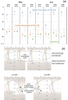
Based on these conclusions, we carried out several numerical experiments during the period from March to July using the described Lagrangian transport model in order to obtain back trajectories of water particles from the Gdask Basin. Since, under the terms of the model, tracers can to move only horizontally within a given layer with a thickness of 4 m, the calculation period begins after the last act of deep vertical mixing before the start of spring warming. According to the data from the Federal Maritime and Hydrographic Agency of Germany (http://www.bsh.de) and the reanalysis of the reviewed years, the last event of deep vertical mixing could be observed in the second half of March (15.03.2004, 23.03.2005, 26.03.2006 Figure 4). The end of backtracking in July corresponds to the date of the field measurements in the Gdask Basin when cold waters with increased salinity had already been identified. The duration of the model calculation was 102–114 days (approximately from March to July). Cross sections from the Arcona to the Gdask Basins (Figure 2, Figure 4) show that vertical mixing falls below 50 m reaching the isopycnal of 9 psu in March. The certain part of the CIL water with the temperature from 1.5 to 3° C and salinity from 7.5 to 9 psu is visible on each section at the depths from 40 to 60–70 m.

Figure 5

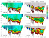
Backtracking results (Figure 5) demonstrated that in the Gdask Basin at depths corresponding to the lower part of the CIL there are tracers that came from the Bornholm Basin and the S{upsk Channel. So the tracks of water particles from the Bornholm Basin are located at the depths from 44 to 64 (2004), from 48 to 64 (2005), and from 52 to 64 m (2006). Tracers from the S{upsk Channel are found at the depths of 64 to 76 m in all years.

Figure 6

The comparison between the back trajectories of water particles and the vertical temperature and salinity profiles from the reanalysis allows us to show that the depth of appearance of the water that came from the southwestern part of the basin coincides with the depth of the lower part of the CIL. That lower part of the CIL has increasing salinity, higher than 7.5 psu but lower than 10 psu, as can be seen from the comparison of the backtracking results and the vertical profiles (Figure 6). However, it can be clearly defined that the considered water mass is not of Atlantic origin because its salinity and temperature are below 10 psu and 5° C, respectively.

4. Conclusions

This study supports the idea of "the spring turnover". The denser water from the southwestern basin of the Baltic Sea renews the lower part of the CIL in its central basins by salty and cold waters after the winter period due to the formation of the salinity gradient in the upper mixed layer. Investigation of the CMEMS reanalysis carried out in this study allowed us to show a rather adequate quality of reproduced structure of the Baltic Sea CIL.

The water characteristics in the Gdask Basin from the reanalysis demonstrate the gradient part of the CIL – the cold waters with the rising salinity that lie above the waters of Atlantic origin. The backtracking analysis points that a certain, part of the Gdask Basin waters from the lower/gradient part of the CIL in summer (in the beginning of July) has been formed by the waters that had come from the Bornholm Basin and the S{upsk Channel after the end of winter vertical convection (in March). The results suggest the same picture in all the considered years (spring–summer 2004–2006). However, the reanalysis results did not directly show that waters entering the central part of the Baltic Sea were renewed from the surface at the end of the winter period. The depths corresponding to the back trajectories of water particles from the Bornholm Basin were deeper than maximums of the mixed layer depths in the considered period. But from the physical point of view, it is clear that the water in the basin moves along the isohalines, which deepen from the southwestern to the northeastern part of the Baltic Sea. However the particles belonging to the gradient sublayer cannot move along the isohalines due to the limitation of the Lagrangian transport model. Accordingly, this study does not directly prove the possibility of renewal of the lower part of the CIL with waters formed during the deep vertical mixing from other basins of the Baltic Sea. Nevertheless, it confirms the general idea of the mechanism of water exchange within the Baltic Proper due to the salinity gradient along its major axis. Obviously this horizontal water transport due to the density gradient inside the basin should work throughout the year. But this effect should make the maximum contribution to the renewal of the lower part of the CIL during the early spring period during the transition from winter to summer.

Acknowledgment

References

Axell, L. (2013) , BSRA-15: A Baltic Sea Reanalysis 1990–2004, Reports Oceanography, 45, p. 55, Swedish Meteorological and Hydrological Institute, Norrköping, Sweden.

Axell, L., Y. Liu (2016) , Application of 3-D ensemble variational data assimilation to a Baltic Sea reanalysis 1989–2013, Tellus A, 68, p. 24220, https://doi.org/10.3402/tellusa.v68.24220.

Chubarenko, I., N. Stepanova (2018) , Cold Intermediate Layer of the Baltic Sea: hypothesis of the formation of its core, Progress in Oceanography, 167, p. 1–10, https://doi.org/10.1016/j.pocean.2018.06.012.

Döös, K., J. Kjellsson, B. Jönsson (2013) , TRACMASS – A Lagrangian trajectory model, Preventive Methods for Coastal Protection, p. 225–249, Springer, New York, https://doi.org/10.1007/978-3-319-00440-2_7.

Funkquist, L., E. Kleine (2007) , HIROMB: An introduction to HIROMB, an operational baroclinic model for the Baltic Sea, Reports Oceanography, 37, p. 36, Swedish Meteorological and Hydrological Institute, SE-601 76 Norrköping, Sweden.

Janssen, F., C. Schrum, J. O. Backhaus (1999) , A climatological data set of temperature and salinity for the Baltic Sea and the North Sea, Deutsche Hydrogaphishe Zeitschrift, Suppl. 9, 51, p. 5, https://doi.org/10.1007/BF02933676.

Hydrometeoizdat, (1992) , V. III. The Baltic Sea, 450 pp., Hydrometeoizdat, Leningrad.

Kapustina, M. V., V. A. Krechik, V. A. Gritsenko (2017) , Seasonal variations in the vertical structure of temperature and salinity fields in the shallow Baltic Sea off the Kaliningrad Region coast, Russ. J. Earth Sci., 17, p. ES1004, https://doi.org/10.2205/2017ES000595.

Korotaev, G. K., V. V. Knysh, A. I. Kubryakov (2014) , Study of formation process of cold intermediate layer based on reanalysis of Black Sea hydrophysical fields for 1971–1993, Izvestiya, Atmospheric and Oceanic Physics, 50, no. 1, p. 35–48, https://doi.org/10.1134/S0001433813060108.

Krechik, V. A., M. V. Kapustina, et al. (2019) , Variability of hydrological and hydrochemical conditions of Gotland and Gdansk Basins' bottom waters (Baltic Sea) in 2015–2016, Russ. J. Earth Sci., 19, p. ES1002, https://doi.org/10.2205/2018ES000641.

Lascaratos, A., W. Roether, K. Nittis, et al. (1999) , Recent changes in deep water formation and spreading in the eastern Mediterranean Sea: a review, Progress in Oceanography, 44, p. 5–36.

Leppäranta, M., K. Myrberg (2008) , Physical Oceanography of the Baltic Sea, 370 pp., Springer, Praxis Publishing, Chichester, UK.

Menna, M., P. M. Poulain (2010) , Mediterranean intermediate circulation estimated from Argo data in 2003–2010, Ocean Sci., 6, p. 331–343, https://doi.org/10.5194/os-6-331-2010.

Oguz, T., S. Besiktepe (1999) , Observations on the Rim Current structure, CIW formation and transport in the western Black Sea, Deep-Sea Research I, 46, p. 1733–1753, https://doi.org/10.1016/S0967-0637(99)00028-X.

Omstedt, A., L. B. Axell (1998) , Modeling the seasonal, interannual, and long-term variations of salinity and temperature in the Baltic proper, Tellus, 50A, p. 637–652, https://doi.org/10.3402/tellusa.v50i5.14563.

Ponomarenko, E. P., V. A. Krechik (2018) , Benthic foraminifera distribution in the modern sediments of the Southeastern Baltic Sea with respect to North Sea water inflows, Russ. J. Earth Sci., 18, p. ES6001, https://doi.org/10.2205/2018ES000632.

Stanev, E. V., M. J. Bowman, et al. (2003) , Control of Black Sea intermediate water mass formation by dynamics and topography: comparisons of numerical simulations, survey and satellite data, J. Mar. Res., 1, p. 59–99, https://doi.org/10.1357/002224003321586417.

Stanev, E. V., J. V. Staneva (2001) , The sensitivity of the heat exchange at sea surface to meso and sub-basin scale eddies. Model study for the Black Sea, Dyn. Atmos. and Oceans, 33, p. 163–189, https://doi.org/10.1016/S0377-0265(00)00063-4.

Staneva, J. V., E. V. Stanev (1997) , Cold water mass formation in the Black Sea. Analysis on numerical model simulations, Sensitivity to Change: Black Sea, Baltic Sea and North Sea, E. Ozsoy and A. Mikaelyan (eds.), NATO ASI Series, Vol. 27, p. 375–393, Kluwer Academic Publishers, Dordrecht, Netherlands.

Stepanova, N. (2017) , Vertical structure and seasonal evolution of the cold intermediate layer in the Baltic Sea, Estuarine, Coastal and Shelf Science, 195, p. 34–40, https://doi.org/10.1016/j.ecss.2017.05.011.

Stepanova, N. B., I. P. Chubarenko, S. A. Shchuka (2015) , Structure and Evolution of the Cold Intermediate Layer in the Southeastern Part of the Baltic Sea by the Field Measurement Data of 2004–2008, Oceanology, 55, no. 1, p. 25–35, https://doi.org/10.1134/S0001437015010154.

Thyng, K M., R. D. Hetland (2014) , TracPy: Wrapping the Fortran Lagrangian trajectory model TRACMASS, Proceedings of the 13th Python in Science Conference (SCIPY 2014), p. 79–84, Austin, Texas, https://doi.org/10.25080/Majora-14bd3278-011.

Tuomi, L., K. Myrberg, A. Lehmann (2012) , The performance of the parameterisations of vertical turbulence in the 3D modelling of hydrodynamics in the Baltic Sea, Cont. Shelf Res., 50–51, p. 64–79, https://doi.org/10.1016/j.csr.2012.08.007.

Umlauf, L., H. Burchard, K. Hutter (2003) , Extending the k-omega turbulence model towards oceanic applications, Oc. Mod., 5, p. 195–218, https://doi.org/10.1016/S1463-5003(02)00039-2.

Received 9 September 2019; accepted 23 January 2020; published 4 June 2020.

 
Citation: Stepanova N., A. Mizyuk (2020), Tracking the formation of the gradient part of the southeastern Baltic Sea cold intermediate layer, Russ. J. Earth Sci., 20, ES3005, doi:10.2205/2020ES000700.
 

Copyright 2020 by the Geophysical Center RAS.