
RUSSIAN JOURNAL OF EARTH SCIENCES, VOL. 20, ES5007, doi:10.2205/2020ES000740, 2020
M. Yu. Reshetnyak1,2
1Schmidt Institute of Physics of the Earth of the Russian Academy of Sciences, Moscow, Russia
2Pushkov Institute of Terrestrial Magnetism, Ionosphere and Radio Wave Propagation of the Russian Academy of Sciences, Moscow, Russia
The size and the age of the inner core impose constraints in modeling of the Earth's core evolution. The origin of the solid core corresponds to the change in convection regime in the core and, correspondingly, to the change in the magnetic field behavior. Meanwhile the standard evolutionary models predict quite young inner core that is not supported by the palaeomagnetic observations, which claim existence of geomagnetic field older than 3 Gy. We solve the inverse problem and find parameters of the model with the inner core older than 3 Gy.
It is believed that the liquid core of the Earth, appeared soon after accretion of the planet, was all the time in the well-mixed state due to the turbulent convection, caused by the superadiabatic heat flux through the core-mantle boundary (CMB) [Gubbins et al., 1979; Labrosse et al., 1997]. The cooling of the mantle, and respectively, the liquid core, leads to the change of convection regime in the core at geological times. After some time the inner core (IC) appears in the center of the Earth and starts to grow due to solidification process. By now its radius $c_m=1220$ km, is 0.35 from the radius of the liquid core. From the origin of IC the pure thermal convection is accompanied by the so-called compositional convection, concerned with solidification of IC.
Due to appearance of two additional energy fluxes at ICB, concerned with compositional convection: the flux of the light constituent and the latent heat flux caused by solidification process, see for details [Braginsky & Roberts,1995]), this kind of convection is three times stronger than the thermal one. As a result, it is supposed, that the origin of IC is the remarkable phenomenon in the history of the Earth, which should change the magnetic field generation essentially.
However, the palaeomagnetic observations do not recognize the IC birth, see review [Reshetnyak and Pavlov, 2016]. This phenomenon, named as the IC paradox [Olson, 2013], can be caused by various reasons, such as the pure knowledge of the initial conditions concerned with accretion, uncertainty in the physical properties of the liquid core under the high pressure, as well as the details of interaction of the liquid core with the mantle, the magnitude of the heat flux at CMB in particular. The more dramatic reason may be related to the specific of the palaeomagnetic observations, based on the assumption of predominance of the dipole field in the past. So far the modern geodynamo models mostly predict that frequent reversals of the field correspond to the non-dipole magnetic field spectrum [Christensen and Aubert, 2006; Driscoll, 2016], we can not exclude this possibility as well.
One of the possibilities to overcome this contradiction is to explore the whole realistic phase space of parameters. Further we firstly check sensitivity of IC evolution to variations of the crucial parameters in the model and discuss underlying physical mechanisms. Secondly, we solve the inverse problem and find parameters, such as CMB heat flux, initial temperature in the center of the Earth, and the solidification temperature, which provide the best correspondence of the inner core's size and age with seismological and palaeomagnetic observations (further the term "inverse problem" is understood in the general sense of the word, namely tuning of the model parameters). For this aim the Monte-Carlo method was used.
We start from the standard evolutionary model of the core developed in [Gubbins et al., 1979], [Labrosse et al., 1997], [Labrosse, 2003]. It is assumed, that initially the liquid core was fully convective. The mantle cooling led to appearance of IC, which size increased from that time significantly, and, perhaps, thermally stratified region near CMB.
The model is based on the large number of parameters and gives distributions of the density, gravity, pressure, temperature, and some other physical properties of the core as a function of the radius and time. Many of them can not be observed directly and should be tested against other theories. As for example, the heat flux at CMB, should be considered together with the processes in the mantle. The electrical and magnetic properties are subject of the geodynamo study. But there is one important exception: the model predicts appearance and growth of IC, which modern radius $c_m$ is estimated by the seismological methods quite accurately.
|
| Table 3 |
Here we start our analysis by checking how variations of some particular parameter influence on $c$, provided all other parameters are constant and taken from [Reshetnyak, 2019], see also Appendix and the Table 3 there.
The other quantity we follow is the birth time of IC $a$, counted from the end of accretion. It can not be estimated directly from observations, however we will discuss its relation to the geomagnetic observations further.
So far cooling of the core is caused by the heat flux at CMB, we start our analysis from dependency of IC growth on this quantity. As was already mentioned, the heat flux can not be measured directly and its magnitude is very uncertain. The most reasonable estimates follow from capability of convection to generate the magnetic field. The pioneer works, based on the simple structures of the large-scale geomagnetic field [Gubbins et al., 1979], [Buffett, 2002] gave the lower estimate of the net heat flux at CMB $Q\sim 2$ TW. Taking into account 3D geodynamo modeling results, which let estimate input of the toroidal and the small-scale counterparts of the magnetic field, increased estimate up to $Q\sim 10\div 20$ TW [Calderwood et al., 2003].
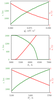 |
| Figure 1 |
Having in mind the above estimates in order of magnitude we introduce the prescribed density flux at CMB as follows $q_b=q_b^\circ(1-0.18 t/A)$, where $\displaystyle q_b=Q/(4\pi r_{CMB}^2)$, $r_{CMB}=3480$ km is the outer core radius, $A=4.5$ Gy is the age of the liquid core, and time $t$ in units of Gy. The resulted IC radius $c$ at $t=4.5$ Gy, and the time $a$ when IC appeared, are shown in Figure 1 (upper plane). The range of $q_b^\circ$ corresponds to the net heat flux $Q$ range at CMB $[12-18]$ TW. The middle value $q_b^\circ=0.075$ mW/m$^2$ corresponds to $15$ TW, used in [Labrosse et al., 1997]. The increase of cooling forces solidification process and as a result $c$ increases, and IC appears faster (small $a$). The less $a$ the older is IC. Its age, measured in Gy, is $4.5-a$. Summarizing, we conclude that increase of $q_b$ in the range $(6\div 9)\, 10^{-2}$ mW/m$^2$ leads to increase of IC radius in the range $(0.84\div 1.4)\,10^3$ km and decrease of $a$ from $3.8$ Gy to $2.5$ Gy.
The next parameter is the initial temperature at $t=0$ in the center of the liquid core $T_\circ$. So far it is assumed that initially core was fully liquid, $T_\circ$ should be larger than the solidification temperature in the center $T_s^\circ$. The estimate of $T_\circ$ is quite uncertain and can rich 10000 K [Rubie et al., 2011]. We adopt more moderate estimate $\sim 6000$ K, used in [Labrosse et al., 1997], [Reshetnyak, 2019]. Variations of $c$ and $a$ are shown in Figure 1 (middle plane). The higher is the initial temperature $T_\circ$ in the center of the Earth the younger is IC, and the smaller is its size. For $T_\circ>6400$ K the core should still be fully liquid.
The last parameter we consider here is the temperature of solidification $T_s^\circ$ in the center of the Earth. Its estimate has been revised in favor of the higher values from $\sim 5270$ K [Labrosse et al., 1997] to $5400\div 5700$ K [Alfé et al., 2007], see in more details [Nimmo, 2007]. Dependencies of $c$ and $a$, as it is expected, see Figure 1 (lower plane), are quite opposite to the previous case with $T_\circ$: increase of $T_s^\circ$ leads to increase of IC size and IC becomes older.
As we can see variations of these three parameters can change IC size and age in wide ranges. These variations cover the acceptable size of IC, as well as predict existence of the quite old IC. The latter reconcile IC evolution with the palaeomagnetic observations, which do not recognize any dramatic change in the geomagnetic field [Reshetnyak and Pavlov, 2016], concerned with IC origin. The further adjustment of the model parameters is the subject of the inverse problem, considered in the next section. The proposed approach is quite general and can be easily extended further.
In spite of the fact that from computational point of view the considered evolutionary model is quite simple, being one dimensional in time and radial coordinate, it is still non-linear because of the properties of the liquid metal, forming the core, depend on the temperature, gravity, which in its turn depend on time. Moreover, complexity of the model is concerned with the threshold phenomena: appearance of two new regions where equations change. The first one is already mentioned IC, which origin leads to the change of the turbulent transport of the heat, described by adiabatic law, to the pure conduction of the heat. The other is appearance of the stably stratified layer at the outer part of the liquid core, where the heat flux can be less than the adiabatic, and again, conduction of the heat takes place [\textcolor{brown}{In all considered cases in Section 2 stable region at CMB was absent.}]. So far the sizes of the both regions can be compared to the size of the liquid core, its influence onto the thermal evolution of the liquid core can be significant.
The mentioned complexity is the reason to explore the full $m$-dimensional space of parameters, where $m$ is the number of varying parameters. For the large $m$, that is the case for the considered model, it can be quite difficult problem, even for a small number of constraints $n$, imposed by observations. As a result special tuning of parameters is needed. Here we present two simple inverse problems of dimension $(m\times n)$, with $m=3$, $n=1$ and $n=2$, solved using the Monte-Carlo method, adopted from the Parker's dynamo simulations, see [Reshetnyak, 2015].
To optimize the selected parameters of the model the following iterative algorithm for the multi-core CPU supercomputer was used. Eqs(1)–(15) were solved numerically with the set ${\cal P}$ of the normally distributed over CPU cores random parameters lying in the prescribed ranges. Using MPI, to the end of the current iteration $M=20$ solutions were obtained, where $M$ was defined by the number of the cores in CPU. To estimate deviation of the simulated solution from the desired one the cost-function $\Psi({\cal P})$ was introduced. By definition the less is $\Psi$ the better solution corresponds to observations. The next iteration starts with the new random $\cal P$ with the mean values of parameters equal to the best choice from the previous iteration and the standard deviation $\sigma=1$. The iterative process stops when $\Psi$ is less than some fixed value, derived from accuracy of observations, either the number of iterations $N$ reaches maximal threshold.
Firstly we considered $(m\times n)=(3\times 1)$ problem with varying ${\cal P}_1=(q_b^\circ,\, T_\circ,\, T_s^\circ)$ and constraint, based on the modern radius $c_m$ of IC. The corresponding cost-function has form:
\begin{equation} \tag*{(1)} \displaystyle{\Psi_1(c_m)=1-e^{-{\cal R}_1},\,\, {\cal R}_1=|c-c_m|.} \end{equation}The closer is $c$ to $c_m$ the "better" is the solution.
 |
| Table 1 |
Using the following ranges of ${\cal P}_1$ $q_b^\circ\in [5\div 9]\, 10^{-2}$ mW/m$^2$, $ T_\circ\in [5\div 7]\, 10^3 $ K, $ T_s^\circ\in [5.1\div 5.7]\, 10^3$ K the evolutionary model was solved $M\times N$ times, where $N\sim 10^4$. The set of the selected solutions after some iterations are listed in the Table 1. The final discrepancy of order $0.1\%$ for $c$ with $q_b^\circ=0.054$ mW/m$^2$ is comparable with accuracy of the seismological observations $\sim 1$ km [Dziewonski and Anderson, 1981]. Even the previous value, corresponding to the higher value of $q_b^\circ=0.074$ mW/m$^2$, does not look unreasonable.
As was already mentioned, appearance of IC leads to the start of compositional convection in the core, release of the large energy, and as a result to the change of geomagnetic field generation. So far there are no supporting palaeomagnetic observations, we can check possibility that in addition IC is quite old [\textcolor{brown}{It is unclear in advance whether the both constraints can be satisfied simultaneously with the desired accuracy.}]. Then the cost-function can be modified as follows:
\begin{eqnarray*} \Psi_2(c_m,\, a) = 1-e^{-{\cal R}_2},\,\, \end{eqnarray*} \begin{equation} \tag*{(2)} \displaystyle {\cal R}_2=w_1|c-c_m|+w_2\theta(a-\hat{a}) |a-\hat{a}|, \end{equation}where $\theta(a-\hat{a})$ is the Heaviside step function, $\hat{a}$ – the desired time when IC appeared, and $w_1=w_2=0.5$ are the weights. The minimum of $\Psi_2$ corresponds to $c=c_m$ and IC older than $\hat{a}$.
 |
| Table 2 |
We considered three regimes with the same set of parameters and ranges as above and the different $\hat{a}$: $1,\, 1.5,\, 2$ Gy, Cases I, II and III, respectively, denoted with the letter "a" in the Table 2.
Only in the Case III, the size of IC $c$ is close to $c_m$ with accuracy 0.3%. The relative accuracy for $a$ is negative $-0.04$, that corresponds to IC older than the proposed estimate $\hat{a}=2$ Gy in 0.08 Gy. Then the age of IC is 2.58 Ga.
As follows from Figure 1 (upper plane), decrease of the heat flux at CMB makes IC older. To demonstrate this we extended range of $q_b^\circ$ to $ [4\div 9]\, 10^{-2}$ mW/m$^2$, see the results in the Table 2, marked by the letter "b". The last two Cases II and III present acceptable accuracy for IC size. In the both Cases $a$ is similar: 1.1 and 1.2 Gy, that corresponds to the age of IC 3.4 and 3.3 Ga, respectively. The estimates in Table 2, give us the range $q_b^\circ=[4\div 5]\, 10^{-2}$ mW/m$^2$, that corresponds to the modern net heat flux $Q$ at CMB in the range $[5.1\div 6.4]$ TW. This range lays between estimates of [Gubbins et al., 1979; [Buffett, 2002] and [Calderwood et al., 2003]. This encouraging result allows us to hope that inclusion of additional optimizable parameters and constraints will help to better understanding of the core evolution process.
Here we considered only a few parameters and constraints, which of course, do not cover all possibilities. Out of scope left the known problem of the radiogenic elements contribution to the energy budget of the core [Labrosse, 2003]. This problem can be solved using the same inverse approach.
The other skipped above non-trivial problem is what happens with the light constituents rising up from ICB to CMB. Usually, in geodynamo models it is assumed that gradient of light constituents at CMB is negligible, that corresponds to the zero flux of the light constituents at the boundary. In its turn it means that compositional convection is suppressed near CMB. In some sense situation is similar to the thermal convection, where the heat flux decreases as $\sim r^{-2}$, but with the additional Neumann boundary condition.
We also did not consider the case of the large thermal conductivity [Pozzo et al., 2012], which can increase adiabatic heat flux at CMB up to 16 TW, forcing development of the thermally stratified layer at CMB. If in addition conductivity increases with the depth, the thermally stratified layer will develop at ICB as well [Labrosse, 2015]. These scenarios also can be tested using above approach in the future.
The author acknowledges financial support from the Russian Science Foundation (grant No. 19-47-04110).
Following [Gubbins et al., 1979], [Labrosse et al., 1997], [Labrosse, 2003] we consider scenario of the Earth's evolution, where soon after the end of the accretion process 4.5 Gy ago, the Earth's core of radius $r_b$ was fully convective. Then, it cooled due to the thermal flux at CMB $r=r_b$, and as a result, depending on the amplitude of the flux $q_b$, two regions could appear: the solid IC ($0\le r\le c$, region I) and subadiabatic layer in the outer part of the core ($r_1\le r\le r_b$, region III) [Gubbins et al., 1982]. The rest convective part of the core $c\le r\le r_1$ here and after is denoted as region II.
Radial distributions of density $\rho(r)$, pressure $P(r)$ and gravity $g(r)$ satisfy to the hydrostatic balance equations:
\begin{equation} \tag*{(3)} \nabla P=-\rho g, \qquad \displaystyle{ g(r)={4\pi G\over r^2} \int\limits_0^r \rho(u) u^2\, du,} \end{equation}with $G$ the gravitational constant. To close system of equations for $(P,\, \rho,\, g)$ the logarithmic equation of state is used:
\begin{equation} \tag*{(4)} P= K_\circ{\rho\over\rho_\circ} \ln {\rho\over\rho_\circ}, \end{equation}where $K_\circ$, $\rho_\circ$ are incompressibility and density at zero pressure, respectively. The optional in the model jump of the density, observed at the surface of the inner core, and which effect on the evolution of the core is quite small, is introduced as follows:
\begin{eqnarray} \tag*{(5)} \rho(r) = \rho(r), \quad \text{if } r \le c \qquad \rho(r) = \rho(r)-\delta\rho, \quad \text{if } r> c. \end{eqnarray}Eqs(3)–(5) with given $c$ we solved numerically, see for details [Reshetnyak, 2019]. Then, with known $(P,\, \rho,\, g)$, adiabatic temperature profile can be derived:
\begin{equation} \tag*{(6)} T_{ad}(r)=T_c(c)\, \exp \left(\displaystyle -\int\limits_c^r {\alpha(u) g(u)\over C_p} \, du \right), \end{equation}where $T_c(c)$ is the temperature at $r=c$, thermal expansion coefficient
\begin{equation} \tag*{(7)} \begin{array}{l} \alpha(r)={\gamma C_p\rho_\circ \over K_\circ\Big( 1+ \displaystyle \ln{\rho\over\rho_\circ} \Big) }, \end{array} \end{equation}with $C_p$ specific heat, and $\gamma$ for Grüneisen parameter.
If IC is still absent, $c=0$, then $T_c(c)=T_\circ$, where the temperature in the center of the Earth $T_\circ$ can be found from the heat balance equation:
\begin{eqnarray*} 4\pi r_1^2 q_1= - 4\pi \int\limits_0^{r_1} \rho C_p {\partial T_{ad} \over \partial t} r^2\, dr=-{\partial T_\circ S \over \partial t}, \end{eqnarray*} \begin{equation} \tag*{(8)} S=4\pi\int\limits_0^{r_1} \rho C_p \, \exp \left(\displaystyle -\int\limits_0^r {\alpha g\over C_p}\right) r^2\, dr, \end{equation}with $q_1$ for heat flux density at $r_1$. The growth of the inner core starts, when temperature of the liquid core is equal to the temperature of solidification:
\begin{equation} \tag*{(9)} T_s(r)=T_s^\circ \left(\displaystyle {\rho(r) \over \displaystyle \rho(c)}\right)^{2(\gamma-{1\over 3 })} , \end{equation}where $T_s^\circ$ is the temperature of solidification in the center of the Earth. Solidification process starts in the core's center, i.e. $T_c=T_\circ=T_s^\circ$, $r=c=0$. Then, for $c>0$, $ T_s$ defines adiabatic temperature at the boundary $c$ in (6): $T_c(c)=T_s(c)$.
Position of the inner core boundary $c$ can be derived from the heat flux equation:
\begin{equation} \tag*{(10)} r_b^2 q_b-c^2 q_c= \dot c \Big( c^2 (P_L+P_G) + P_C \Big), \end{equation}where on the left side is the total heat flux in the region II, and on the right one are the cooling sources, and the dot over $c$ stands for the time derivative.
The latent heat source is defined as
\begin{equation} \tag*{(11)} P_L(c) = \rho(c)\delta S\, T_s(c), \end{equation}with $\delta S$ entropy of crystallization.
Estimate of the release of the gravitational energy due to the growth of the inner core has the form [Loper, 1984]:
\begin{equation} \tag*{(12)} E_G= {2\pi \over 5} G M_\circ \delta \rho {c^3\over c_b} \left(1-\left({c\over r_b}\right)^2 \right), \end{equation}with mass of the core $\displaystyle M_\circ=4\pi\int\limits_0^{r_b}\rho(r) r^2\, dr$ constant in the model. Then it leads to
\begin{equation} \tag*{(13)} \dot E_G=P_G\dot c, \quad P_G={12\pi\over 5} {G M_\circ\delta\rho\over r_b} c \left(1-{2c^2\over r_b^2}\right). \end{equation}The main term, concerned with adiabatic cooling, has the form:
\begin{equation} \tag*{(14)} P_C = - \int\limits_c^{r_1}\displaystyle \rho C_p {\partial T_{ad} \over \partial c} r^2\, dr,\qquad dc\equiv dr, \end{equation}with $q_c$ heat flux density through the boundary $c$. Eq(11) was resolved with respect to $\dot c$ and then integrated in time. This defines evolution of the inner core boundary $c$ in time.
From condition of continuity of the temperature at the boundary $c$, follows that $T_s(c)$ is the boundary condition for the thermal-diffusion equation in the region I, with a moving boundary $c(t)$ [Kutluay, 1997]
\begin{equation} \tag*{(15)} {\partial T\over \partial t}=k \Delta T, \end{equation}where $k$ is the thermal diffusivity. The second boundary condition in the center $r=0$ is $T'=0$, where $'$ is a derivative on $r$. The joined system (1)–(15) defines evolution of the fields in the regions I and II.
If the adiabatic heat flux density $\displaystyle q_{ad}(r) =$ $\displaystyle -\kappa T'_{ad}(r)$, with thermal conductivity $\kappa=k\rho C_P$, becomes larger than the heat flux density at the outer boundary $r_b$: $\displaystyle q_{ad}(r)<\left( {r_b\over r } \right)^2 q_b$, the subadiabatic stably stratified thermal region III develops at the outer part o the core, where the heat flux density is smaller. The temperature profile in the region III can be derived from Eq(12) with the moving boundary $r_1(t)$, and two boundary conditions: $T(r_1)=T_{ad}(r_1)$ at the inner boundary, and given heat flux density $q_b(t)$ at the outer boundary $r_b$. In the general case Eqs(1)–(15) in regions I–III are solved numerically, using iterative methods with under-relaxation method to provide numerical stability. The numerical values of parameters are listed in the Table 3.
The developed MPI C++ code provides possibility to solve equations for the set of parameters simultaneously, as well as to solve the inverse problem using the Monte-Carlo method, similar to [Reshetnyak, 2015]. The Matplotlib Python library was used for graphics. The 40-cores workstations Intel(R) Xeon(R) CPU E5-2640 with Gentoo OS were used for simulations.
Alfé, D., M. J. Gillan, G. D. Price (2007) , Temperature and composition of the Earth's core, Contemp. Phys., 48, no. 2, p. 63–80, https://doi.org/10.1080/00107510701529653.
Braginsky, S. I., P. G. Roberts (1995) , Equations governing convection in Earth's core and the geodynamo, Geophys. Astrophys. Fluid Dyn., 79, no. 1–4, p. 1–97.
Buffett, B. A. (2002) , Estimates of heat flow in the deep mantle based on the power requirements for the geodynamo, Geophys. Res. Lett., 29, no. 12, p. 1566-7-1–1566-7-4, https://doi.org/10.1029/2001GL014649.
Calderwood, A., P. Roberts, C. Jones (2003) , Energy fluxes and ohmic dissipation in the Earth's core, Earth's Core and Lower Mantle. Series: The Fluid Mechanics of Astrophysics and Geophysics. Eds. K. Zhang, A. Soward, C. Jones., 68, p. 100–129, https://doi.org/10.1201/9780203207611.ch5.
Christensen, U. R., J. Aubert (2006) , Scaling properties of convection-driven dynamos in rotating spherical shells and application to planetary magnetic fields, Geophys. J. Int., 166, p. 97–114.
Driscoll, P (2016) , Simulating 2 Ga of geodynamo history, Geophys. Res. Lett., 43, no. 11, p. 5680–5687, https://doi.org/10.1002/2016GL068858.
Dziewonski, A. M., D. L. Anderson (1981) , Preliminary reference Earth model, Phys. Earth Planet. Int., 25, p. 297–356.
Gubbins, D., T. G. Masters, J. A. Jacobs (1979) , Thermal evolution of the Earth's core, Geophys. J. R. Astron. Soc., 59, no. 1, p. 57–99.
Gubbins, D., C. J. Thomson, K. A. Whaler (1982) , Stable regions in the Earth's liquid core, Geophys. J. Int., 68, p. 241–251.
Kutluay, S., A. R. Bahadir, A. Özde (1997) , The numerical solution of one-phase classical Stefan problem, J. Comp. App. Math., 81, p. 135–144.
Labrosse, S., J. P. Poirier, J.-L. Le Mou{ë}l (1997) , On cooling of the Earth's core, Phys. Earth Planet. Int., 99, p. 1–17.
Labrosse, S. (2003) , Thermal and magnetic evolution of the Earth's core, Phys. Earth Planet. Int., 140, p. 127–143.
Labrosse, S. (2015) , Thermal evolution of the core with a high thermal conductivity, Phys. Earth Planet. Int., 247, p. 36–55, https://doi.org/10.1016/j.pepi.2015.02.002.
Loper, D. E. (1984) , Structure of the Core and Lower Mantle, Adv. Geophys., 26, p. 1–34.
Nakagawa, T. (2018) , On the thermal-chemical origin of the stratified region at the top of the Earth's core, Phys. Earth Planet. Int., 276, p. 172–181, https://doi.org/10.1016/j.pepi.2017.05.011.
Nimmo, F. (2007) , Energetics of the Core, Treatise on Geophysics, p. 431–432, https://doi.org/10.1126/science.1243477.
Olson, P. (2013) , The new core paradox, Science, 342, no. 6157, p. 431–432, https://doi.org/10.1126/science.1243477.
Pozzo, M., C. Davies, D. Gubbins, D. Alfé (2012) , Thermal and electrical conductivity of iron at Earth's core conditions, Nature, 485, p. 355–358, https://doi.org/10.1038/nature11031.
Reshetnyak, M. Yu., V. E. Pavlov (2016) , Evolution of the Dipole Geomagnetic Field. Observations and Models, Geomagn. Aeronom., 56, no. 1, p. 110–124, https://doi.org/10.1134/S0016793215060122.
Reshetnyak, M. Yu. (2015) , Inverse problem in Parker's dynamo, Russ. J. Earth Sci., 15, p. ES4001-1–ES4001-7, https://doi.org/10.2205/2015ES000558.
Reshetnyak, M. Yu. (2019) , Evolution of the inner core of the Earth: consequences for geodynamo, Magnetohydrodynamics, 55, no. 1–2, p. 175–183, https://doi.org/10.22364/mhd.55.1-2.21.
Rubie, D. C., D. J. Frost, U. Mann, et al. (2011) , Heterogeneous accretion, composition and core–mantle differentiation of the Earth, Earth Planet. Sci. Lett., 301, p. 31–42, https://doi.org/10.1016/j.epsl.2010.11.030.
Received 13 September 2020; accepted 17 September 2020; published 22 September 2020.

Citation: Reshetnyak M. Yu. (2020), Inverse problem for the Earth's core evolution model, Russ. J. Earth Sci., 20, ES5007, doi:10.2205/2020ES000740.
Copyright 2020 by the Geophysical Center RAS.