
RUSSIAN JOURNAL OF EARTH SCIENCES, VOL. 20, ES1001, doi:10.2205/2019ES000684, 2020
V. N. Kozhevnikov1, R. B. Berzegova2, M. K. Bedanokov2
1Lomonosov Moscow State University, Moscow, Russia
2Maykop State Technological University, Maykop, Russia
[1] The Novorossiysk bora is being studied for the first time as a phenomenon of flowing around real low mountains using a nonlinear analytical two-dimensional model. The vertical unboundness of the atmosphere is taken into account in a three-layer representation, characteristic features of the relief shape are considered exactly, the kinematics and the dynamics of the interaction of flows in different layers are considered approximately. The role of the magnitude of the flow velocity with its characteristic hydrostatic stability is being investigated for the first time in a wide range. It has been shown for the first time that disturbances over real low mountains can remain significant at altitudes of 30 km; Long's resonance effects in the troposphere are excluded; the dependence of the disturbances on the velocity has a decreasing character only on average, and for some velocity values it has a wave character. The conditions for the appearance of rotors in the flow and degree of their stability in the presence of stratification are being discussed.
The work continues to study disturbances that occur in the atmosphere when flowing around mountains of real form based on analytical modelling. A non-linear stationary two-dimensional meso-scale open model is used: velocity disturbances are considered without simplifications, Coriolis forces are not considered, the vertical unboundness of the atmosphere is considered in a three-layer version, in which the lower layer represents the troposphere, and the other two- the influence of the upper atmosphere [Kozhevnikov, 1999, 2019]. The validity of this approach is confirmed by the works [Gutman, 1969; Kozhevnikov, 1970, 1999, 2019; Long, 1955]. The aim of the work is to study not only general properties of disturbances, but their local features, leading to catastrophic destruction during a bore in the area of Novorossiysk city. In this case the experience of using the model for other mountain areas is considered [Berzegova and Bedanokov, 2018; Berzegova et al., 2017; Bedanokov et al., 2018; Kozhevnikov, 2019; Kozhevnikov and Bedanokov, 1993, 1998; Kozhevnikov and Pavlenko, 1993]. The dependence of disturbances on the properties of an incident flow is being studied for the first time in a wide range of its changes.
Analysis of the work [Bedanokov et al., 2018] showed that when conducting similar studies, numerical models are also used [Durran, 1986; Efimov and Barabanov, 2013; Gavrikov and Ivanov, 2015; Lin, 2007; Toropov et al., 2013; Toropov and Shestakova, 2014; Shestakova et al., 2015]. They take into account more physical factors than in analytical models, but this is done through the use of a number of parametric ratios. The derivatives in the equations here are replaced by finite differences, the problem of reliable accounting of the initial and boundary conditions is also complicated. It turns out that, despite many advantages, it is always difficult to determine uncertainty that approximations bring to the results when analyzing the results of the use of such models. Hence, when studying the problem posed, it is necessary to use both analytical and numerical modelling methods.
The simulation of the mountain flow was carried out on the basis of the solution of the Helmholtz equation for disturbance stream function [Kozhevnikov, 1999, 2019]:
\begin{eqnarray*} \nabla^2 \psi' + K^2 \psi' =0, \quad \psi' = \psi - \psi_0 \end{eqnarray*} \begin{equation} \tag*{(1)} \psi_0= - Uz, \quad K= \frac{N}{U}= 2 \pi \lambda_c^{-1} \end{equation}\begin{eqnarray*} N^2 = \frac{g}{\Theta} \frac{d \bar{\Theta}}{dz} = \frac{g(\gamma_a - \gamma)}{T_1}, \quad \gamma= - \frac{d \bar{T}}{dz} \end{eqnarray*} \begin{eqnarray*} \lambda_c = 2 \pi \frac{U}{N}, \quad \Theta = T \Bigl( \frac{p_0}{p} \bigr)^{(k-1)/k}, \quad \end{eqnarray*} \begin{equation} \tag*{(2)} \nabla^2 = \frac{\partial^2}{\partial x^2} + \frac{\partial^2}{\partial z^2} \end{equation}
where $\psi$, $\psi'$, $\psi_0$ stream function, its disturbances and its values in an undisturbed incident flow in front of the mountains, where $U$ velocity and $\gamma$ gradient are given. Besides, here: $x, \; z$ are horizontal and vertical coordinates in the considered vertical plane, $N$ is Brent-Väisäl wave frequency, $\lambda_c$ is Lira wave scale [Lyra, 1943], $\Theta$ is a potential temperature, $\gamma$, $\gamma_a$ are vertical and dry adiabatic temperature gradients, $T$ is temperature, $T_1$ representative (average) temperature of a layer, $g$ is gravity acceleration, $k$ is relation of specific thermal capacities. The values characterizing the parameters of the incident flow in front of the mountains are highlighted with an over-line. Temperature disturbances $T'(x,z )$ are calculated by the formula:
\begin{equation} \tag*{(3)} T' = \frac{(\gamma_a - \gamma) \psi'}{U} \end{equation}Velocity components are defined by the derivatives of $\psi$ vertically and horizontally. Ratios (1)–(3) are obtained from a system of well-known nonlinear equations of state, motion, continuity, and thermodynamics using assumptions about adiabaticity, incompressibility, absence of viscosity and Coriolis forces. Nonlinearity of the velocity field is considered due to some particular case [Gutman, 1969; Kozhevnikov, 1999]:
\begin{eqnarray*} U= \mathrm{const}, \quad \gamma = \mathrm{const} \end{eqnarray*}As the model is two-dimensional, the streamlined relief should have a cylindrical character, and its shape should be defined by a profile in a vertical plane $(x,z)$, oriented towards the incident flow. The model considers the specified shape of the contour interval within the accuracy of ten meters. The conditions of kinematic and dynamic conjugation of flows on the interfaces of the layers are linearized (set on fixed horizontals) [Kozhevnikov, 1999; Kozhevnikov and Bedanokov, 1993]. The model makes it possible to vary the parameters of the problem smoothly, while $U$ is assigned with the same value in all layers, and $\gamma$ is assigned with different ones. The previous experience of using the model has shown that disturbances primarily depend on the $\lambda_c$ scale, and according to (2) it directly depends on $U$ and less on $\gamma$. At this stage, it has been decided to carry out basic calculations for 11 options for setting the $\lambda_c$ scale in the troposphere and for one option for setting layer-by-layer values (bottom up $j = 1, 2, 3$):
\begin{eqnarray*} \lambda_c =3, 4, 5, 6, 6.66, 7, 7.5, 7.8, 9.5, 10, 12.2\; \mathrm{km}, \end{eqnarray*} \begin{equation} \tag*{(4)} \gamma_j=6, 0, 3 \;\mathrm{grad/km} \end{equation}Further, the values of $\lambda_c$ are assigned in km, and that of $\gamma$ in grad/km. The assigned values of $\lambda_c$ variations correspond to $U$ variations in the range from 6 to 24.4 m/s. The greatest values of $U$ in (4), for sure, are of little practical value, but they are important for theoretical reasons. The heights of the interfaces have been assigned with values of 10 and 18 km, the calculations have been carried out to the height of 30 km. At $\lambda_c$ variation, Long's conclusion [Long, 1955] has been taken into account that in closed models the solution loses its meaning when a half of $\lambda_c$ fits into the vertical thickness of the flow a whole number of times. It has been shown in [Kozhevnikov, 1970, 1999] that this effect is determined by the excitation of a resonance in the considered liquid layer. In order to quantify the presence of this effect in the troposphere, a provision has been made to include $\lambda_c$ the values of $\lambda_c = 4, 5, 6.66$ and 10 in (4), at which 1/2 of $\lambda_c$ fits into the troposphere thickness 5, 4, 3, 2 times.
Theoretically, the entire half-space in the vertical plane, bounded from below by the relief section, is considered. The calculations were carried out vertically up to 30, horizontally in the range $- 30 < x < +40$ km. It was taken into account that the inflowing stream at infinity in front of the mountains is not disturbed. The classical conditions of dynamics and kinematics were realized on the interfaces of the layers and on the streamlined surface of the earth. In this case: a) the conditions on the interface were linearized, since they were placed on the horizontals, the height of which is determined in the flowing stream; b) the conditions on the ground are fulfilled with the required accuracy (in accordance with today's practice requirements). In the upper layer, the assumption was used that the wave energy of disturbances propagates only upward. In the leeward region beyond the mountains, no restrictions were imposed.
To take into account the dependence on the horizontal coordinate, the Fourier method is used in the solution (1). Spectral composition of wave components of the solution depends on all the parameters of the problem, but primarily on $\lambda_c$ and the shape of the streamlined mountains. The solution has the form of complex functionals, that include integrals over the horizontal coordinate and wave numbers. In the latter case, wavelengths greater than 3 km were taken into account. It is important that when the position of the calculation point in space and the parameters of the problem change, the result changes smoothly, singularity-free. The computational grid steps for calculating the field make 50 m and 250 m along $x$ and $z$, respectively, which ensures a high quality of spatial resolution.
|
| Figure 1 |
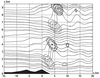
The relief of Novorossiysk outskirts is illustrated by the isohypses of heights presented in Figure 1. For their construction, data obtained on the basis of the digital terrain model ETOPO2 (Digital relief model ETOPO2 [Electronic resource], Access mode: http://www.ngdc.noaa.gov/mgg/global/rel ief/ETOPO2/, free) were taken. We used an array of heights with a latitude and longitude resolution of 30 seconds (about 0.9 in latitude and 0.7 km in longitude). The mountains here are represented, on average, by two ranges parallel to the coast. The position of the coastal range is shown in the figure by a hatched line, and the direction of the vertical plane of modeling by a continuous one. The latter is perpendicular to the set of the hills and coincides with the direction of the northeast winds at bore. To highlight two-dimensional features of the relief, a special processing program for the specified array has been created. At first, changes in the altitudes have been determined, which define two-dimensional features of the $h(x)$ relief along 10 sections in the vertical modeling plane, shifted from each other by 0.9 km. The characteristics of the dominant ridges and hollows of the mountains have been considered as defining features. This principle has been used successfully in [Bedanokov et al., 2018; Berzegova and Bedanokov, 2018; Berzegova et al., 2017; Elansky et al., 2003; Kozhevnikov, 1999, 2019; Kozhevnikov and Pavlenko, 1993; Kozhevnikov and Bedanokov, 1993, 1998; Kozhevnikov et al., 1986, 2017].
 |
| Figure 2 |
The obtained $h(x)$ arrays have been used to determine the averaged sectional shape of the $sr$ relief. The obtained averaged sr profile is shown in Figure 2 solid bold line. To identify the effect of changes in the shape of the relief on the disturbances, an $h(x)$ array was also considered in which the main heights differed noticeably from the heights of $sr$. We will call it quotient and denote as $ch$. An important feature of these sections is the presence of two dominant ranges and a deep hollow between them. To assess the impact of these particular features, two artificial reliefs with one dominant range have been created.
 |
| Table 1 |
We will designate them as $iskV$ and $iskN$. Important characteristics of all sections are given in Table 1.
They have the same area (with an accuracy of 7.6%) and the steepness of the leeward slope of the coastal range is almost the same.
 |
| Figure 3 |
 |
| Figure 6 |
 |
| Figure 4 |
3.2.1. First of all, 44 variants of flow have been calculated and analyzed in accordance with (4). In the analysis, two figures were considered each time – for heights up to 30 and 12 km and $-30
3.2.2. When comparing the results for $sr$ and $ch$ reliefs, it has been established that the trajectory fields do not differ qualitatively. This has made it possible to investigate the basic properties of disturbances by analyzing the results for $sr$ only.
3.2.3. The areas of $T'$ are arranged in a certain order in space in the form of oval spots and they show that disturbances are not just wave-like, but form peculiar repeating structures [Kozhevnikov, 1999, 2019]. Spots of a different $T'$ sign are located in different height ranges, repeating with a period close to $\lambda_c$. At fixed heights, the location of spots downstream repeats periodically, but with a period that may differ significantly from $\lambda_c$. In [Bedanokov et al., 2018; Berzegova and Bedanokov, 2018; Berzegova et al., 2017; Kozhevnikov, 1999, 2019; Kozhevnikov and Pavlenko, 1993; Kozhevnikov and Bedanokov, 1993, 1998; Kozhevnikov et al., 1986] attention has already been paid to the fact that not only the $\lambda_c$ scale manifests itself in disturbances, but so does the scale of change in the shape of the relief. The results of this research, confirm the abovementioned facts and draw attention to the following. 1) The scale of the mountain shape can directly manifest itself in the field of trajectories: in Figure 3 trajectories with $z_0 =1.25$ and 2.75 follow closely the shape of the mountains – the first one in an inverted form, the second – directly. 2) Areas of abrupt accumulation of trajectories – jet streams – appear periodically over the mountains. 3) The presence of two rather distant from each other ranges gives rise to two almost independent disturbance systems over the mountains.
3.2.4. The fields of $T'$ have made it possible to establish that the initial hydrostatic stability over the mountains varies slightly. Calculations for $\lambda_c= 3$ have shown that in the area of $T'>0$ above the lee slope of the mountains (Figure 4, the area of the point of $x = 1.7$, $z = 1.2$ km), $\gamma$ gradient increases by 15% slightly higher above the center compared to the background value and becomes 6.9, and slightly lower it decreases by 30% and equals to 4.2. It is obvious that in other cases these changes are less.
3.2.5. According to Figure 2, Figure 3 the rotors appear above the mountains with a value of $\lambda_c = 3$, i.e. in [Long, 1955] the area where air particles move either vertically or even towards the main flow. In [Kozhevnikov, 1963, 1965, 1968, 1999, 2019; Mailes, 1968], when discussing this problem, the reciprocal of the internal Froude number is being considered, in which the maximum height of $h_m$ mountain is used as the scale. In accordance with [Lin, 2007], we call it dimensionless mountain height and define it as the relations of:
\begin{equation} \tag*{(5)} \zeta = F^{-1}_i = \frac{N h_m}{U} = 2 \pi \frac{h_m}{\lambda_c} \end{equation}
In this research the specified parameters vary within:
\begin{eqnarray*} 0.87 < F_i <3.59, \quad 1.14 < \zeta < 0.28 \end{eqnarray*}Figure 4 represents disturbance pattern for $\lambda_c =5$, that is considered to be typical for the atmosphere. A comparison of the presented trajectory fields shows the extent at which disturbances attenuate when $\lambda_c$ increases. At $\lambda_c =3$ the rotors are observed over the leeward slopes of both ranges and they periodically repeat at all considered heights, i.e. up to 30 km. In Figure 4 the rotors are visible only in the area behind the last range along the stream and not in the first height range, but in the second one. With values of $\lambda_c >5$ the rotors are missing.
Therefore, in accordance with (5), rotors appear at $\zeta$ values equal to or greater than 0.69, or $F_i$ values less than or equal to 1.45. In [Kozhevnikov, 1963, 1965, 1968, 1999; Mailes, 1968] for a semicircle mountain with a height of 1 km, the critical value of $\zeta$ lay in the range of 1.27–1.5. In our case, the relief has a height of $h_m = 0.548$ km and is much longer. In accordance with (5), the critical value of $\zeta$ should lie in the range of $\zeta =(1.27 - 1.5) \times 0.548=(0.69 - 0.72)$ due to reducing the height. This means that the critical value of $\zeta$ depends primarily on $h_m$. In [Kozhevnikov, 1965, 1999; Kozhevnikov and Pavlenko, 1993] it has been concluded that the intensity of the disturbances depend on the characteristics of the shape of the mountains in order of importance: the height, the steepness of the leeward slope, the sectional area. The sectional area in our case was significantly larger than the area of the semicircle. Hence, the steepness of the investigated mountains affected the disturbances in the same way as the steepness of the semicircle mountain. A number of authors believe that determined critical values of $\zeta$ can be used as a sign of a "wave breaking" process beginning. In [Shestakova et al., 2015; Toropov and Shestakova, 2014; Toropov et al., 2013] some of the obtained results are also interpreted as a prediction of the effect of "breaking" of waves, that is, the transformation of the laminar wave flow into a purely turbulent one. However, this is done without convincing evidence. In [Efimov and Barabanov, 2013] the proximity of the slope of isolines of the potential temperature to the vertical is used as a criterion for "wave breaking". Although this approach qualitatively coincides with the above reasoning about the rotors, it does not give quantitative ratios. For now, we can't say how obtained estimates of the critical value of $\zeta$ are applicable to determine the beginning of the rotor "breaking" process in the nature. In [Long, 1955] Long proposed to consider the appearance of rotors as a sign of the loss of the model representativeness. However, his experiments proved that developed rotor circulations existed stably, and this meant that the real stability of fluid motions could significantly increase in the presence of density stratification in it. In [Kuttner, 1958] the fact of the frequent and stable existence of such rotors in nature was established. In [Kozhevnikov, 2019] a comparison of the calculations for this model with direct measurements has shown that the stability of rotor circulations is rather underestimated. It is quite possible to assume that, in the areas of rotor prediction, such variants are possible, as: a steady laminar flow, appearance of local sources of turbulence, a complete "wave breaking".
 |
| Figure 5 |
 |
| Table 2 |
3.2.6. Earlier in [Bedanokov et al., 2018; Berzegova and Bedanokov, 2018; Berzegova et al., 2017; Kozhevnikov, 1963, 1965, 1968, 1999, 2019], it was found using a number of examples that the intensity of perturbations decreases with increasing of $\lambda_c$ . This property will be called the smoothing regularity. Figure 3–Figure 5 shows this trend by the example of two values of $\lambda_c$. The analysis of the results obtained for the entire range (4) has revealed that if the disturbances in the leeward region depend on $\lambda_c$ linearly, then the dependence over the mountains is more complex and it can be, for example, illustrated by maximum values of the range of vertical displacements of $\Delta (\psi'/U)$ trajectories from the original levels of $z_0$ and with extreme values of $T'$ (in degrees). These dependences are shown in Table 2, where the lines from top to bottom show the values: $\lambda_c$, $z_0$ for trajectories with maximum displacements, $\Delta (\psi'/U)$, extreme $T'$ (in degrees). We can see that the amplitudes of $\Delta (\psi'/U)$ begin to decrease at $\lambda_c$ equal and larger than 4 above the mountains. However, a little further the trend changes, and all the amplitudes of the displacements begin to increase in the range of changes from 7.8 to 9.5. Specifically, at $\lambda_c=9.5$ the maximum of amplitudes returns to the level that occurred at $\lambda_c = 6.66$. If the increase of continues, the previous smoothing trend restores. The disturbances $T'$ demonstrate a similar dependence. The $\psi$ field at $\lambda_c=12.2$ has the form of classical waves everywhere, the amplitude of which does not exceed 0.5 km, and the length is close to the value of $\lambda_c$. The physical meaning of this regularity is not yet completely clear.
Apparently, the linear dependence is determined by the fact that the increase of $\lambda_c$ is associated, foremost, with an increase in $U$ speed and, therefore, a decrease in the time of interaction of the moving atmosphere with the uneven ground, i.e. with a decrease in the energy effect of the relief on the flow (see [Gill, 1986], Vol.1, i.8.8). Deviation from linearity is apparently determined by the processes of energy interaction between the selected layers, and they have to be investigated yet.
3.2.7. Additional calculations have been carried out for 2 variants of the flowing in order to estimate how much the results can change if $\gamma$ gradients differ from the values provided for in (4). Here, the scale values of $\lambda_1$ have been set the same and they are equal to 5, and $\gamma$ values in the troposphere different by $+/- 1$ degrees/km as compared to the former $\gamma = 6$. The corresponding values of $U$ became equal to 8.7 and 11.1.
Comparison of the obtained results with the previous one (Figure 5) has shown that the fields of $\psi$ in the troposphere in 3 variants are almost the same. It turns out that the results obtained for the troposphere by setting (4) are valuable not only for situations with a gradient of $\gamma_1=6$, but also for the cases when this gradient is different from that indicated by 1–2 degrees/km, i.e. for a wider range of stability values of the incident flow.
3.2.8. The range (4) included $\lambda_c$ values at which, according to Long [Kozhevnikov, 1970, 1999; Long, 1955], one would expect resonance excitation in the troposphere. It was established that there was no noticeable increase in disturbances at such values of $\lambda_c$. Consequently, with typical changes in the stability from the troposphere to the stratosphere, the reflection of wave energy from the upper layers downwards is always partial, and therefore, according to Long, resonance effects in the troposphere are excluded.
3.2.9. Comparison of the results for $sr$ and $iskV$ at $\lambda_c=5$ has shown that the presence of a hollow between two ridges leads to a noticeable increase in disturbances in the most noticeable crests of waves over the mountains and at the beginning of the leeward zone. The trajectory with $z_0= 7.5$ has the range of vertical displacement 38% more than in case of one spinal relief.
Additionally, this trajectory acquires a completely rotor character. Comparing the data for the $iskV$ and $iskN$ reliefs, one can see how the range of the trajectory displacement decreases by about 28% as the mountain height decreases. It has been estimated that the maximum range of vertical displacements of air particles in the troposphere is related to the maximum height. According to [Kozhevnikov, 1999], at $\lambda_c=5.1$ the indicated range above the mountains of the Crimea has been 3.6 in fractions of height. According to the results of this research, it has been for a smaller value of $\lambda_c : 2.8$ is for an average relief (Figure 4), 1.1 is for $iskV$ relief, 0.4 is for $iskN$ relief. Once again it is confirmed that the intensity of the disturbances primarily depends on the height of the mountains and secondly on their shape.
3.2.10. The simulation results presented in Figure 3 and Figure 6 show that the intensity of disturbances in the upper layers is very high and it weakens slowly with height. The amplitudes of vertical displacements of air particles at altitudes of 20–30 km are typically close to $h_m$. It has been shown for the first time for relatively low mountains, i.e. occurring quite often on the earth.
In 5 out of 11 analyzed variants, orographic waves are developed in all upper layers and at both interfaces. In 2 cases the waves are developed in the 3rd layer and at the 2nd interface. In 4 cases, the waves are almost undeveloped in the upper layers and at both interfaces. It has been established that in each upper layer the amplitudes of the waves are determined primarily by the disturbance at its lower boundary, i.e. in each overlying layer the air stream flows around a sort of "its own mountain". The height of such "mountains" on the surfaces of the interface becomes noticeable when in the underlying layer the height of the upper boundary of the latter coincides with the level of maximum amplitudes due to the periodicity of vertical changes.
The results of additional calculations analyzed partially in p. 2.7 have shown that the intensity of disturbances in the upper layers depends on the level of reflection of wave energy at the interfaces of the layers. Figure 6 shows the trajectories of movement in layers 2 and 3 in variants that differ only in values of in the troposphere: a thin continuous line for $\gamma = 6$ and a thick dashed line for $\gamma=5$.
We can see that the disturbances in the upper layers in the second case have increased by no less than two times. Here, the scale of $\lambda_c$, although it has increased slightly everywhere, hasn't noticeably changed the nature of the disturbances, in particular, the trajectories in the tropopause area have remained almost unchanged and have been slightly disturbed. In the variant with smaller $\gamma$ disturbances in the upper layers have increased, apparently, due to a decrease in the wave energy reflection at the tropopause (the gradient changed less during the transition from the troposphere to the stratosphere).
3.2.11. The disturbances quickly become wavelike in the lower layers of the troposphere in the leeward region, as they move away from the mountains, and the waves abate slowly along the flow. These results are of only qualitative interest, since viscous forces have not been considered in the model. When $\lambda_c$ increases, these properties almost do not change, only the height and wavelength change. In particular, the following has been established. Wave amplitudes at altitudes of about 0.5 km at $\lambda_c=3$ are noticeable at distances from mountains up to 27 km and are degenerated at large values of the Lyra scale. At altitudes of 1 km they are noticeable: up to 31 km at $\lambda_c=3$, up to 28 km at $\lambda_c=5$, up to 20 km at $\lambda_c = 6$ and further they become trivial.
It was shown for the first time that, when flowing around, real mountains of small height very strongly disturb the atmosphere not only at all levels in the troposphere, but also at altitudes of the order of 30 km. This result is important because it is widely believed in the literature that the vertical scale of the Novorossiysk pine forest is limited to one two kilometers. For the first time, the dependence of perturbations on the properties of a leaking stream in a wide range of its properties is investigated. For the first time, it has been quantitatively shown that Long resonance is excluded in the troposphere, since the reflection of wave energy from the upper layers is not complete. It is shown that the previously approximately formulated regularity of smoothing disturbances with an increase in the wave scale is fulfilled only on average for Novorossiysk boron and deviations from it can be noticeable.
Berzegova, R. B., M. K. Bedanokov (2018) , Disturbances of the atmosphere during the flow around the mountain ranges, Izvestiya. Atmospheric and Oceanic Physics, 54, no. 5, p. 534–545, https://doi.org/10.1134/S0001433818050043 (in Russian).
Berzegova, R. B., M. K. Bedanokov, S. K. Kuizheva (2017) , Atmospheric Disturbances in the Airflow around Mountains and the Problem of Flight Safety in the Mountains of the Republic of Adygeya, Ecologica Montenegrina, 14, p. 136–142.
Bedanokov, M. K., R. B. Berzegova, et al. (2018) , A review of the works devoted to modeling the phenomena of flow around asperities of the earth and catastrophic winds of the bora type, Vestnik of TvSU. Series "Geography and Geoecology", 3, p. 15–39 (in Russian).
Durran, D. R. (1986) , Another look at downslope windstorms. Part I: The development of analogs to supercritical flow in an infinitely deep, continuously stratified fluid, J. Atmos. Sci., 43, p. 2527–2543, https://doi.org/10.1175/1520-0469(1986)043%3C2527:ALADWP%3E2.0.CO;2.
Gavrikov, A. V., A. Y. Ivanov (2015) , Anomalously strong bora over the Black Sea: Observations from space and numerical modeling, Izvestiya. Atmospheric and Oceanic Physics, 51, no. 5, p. 546–556, https://doi.org/10.1134/S0001433815050059.
Gill, A. (1986) , Dynamics of the Atmosphere and the Ocean, v. 1–2, Mir, Moscow.
Gutman, L. N. (1969) , Introduction to the Nonlinear Theory of Mesomereteological Processes, 295 pp., Hydrometeoizdat, Moscow.
Efimov, V. V., V. S. Barabanov (2013) , Modeling of the Novorossiysk bora, Meteorology and Hydrology, 3, no. 3, p. 171–176, https://doi.org/10.3103/S1068373913030059 (in Russian).
Elansky, N. F., et al. (2003) , Effect of orographic disturbances on ozone redistribution in the atmosphere by the example of airflow about the Antarctic Peninsula, Izvestiya. Atmospheric and Oceanic Physics, 39, no. 1, p. 93–107.
Kozhevnikov, V. N. (1963) , On a nonlinear problem of the orographic disturbance of a stratified air flow, Izv. of the USSR Academy of Sciences. Ser. Geophysics, 7, p. 1108–1116.
Kozhevnikov, V. N. (1965) , Orographic Disturbances of the Air Flow, Dissertation for the degree of Cand. of Phys.-Math. sc., MSU, Faculty of Physics, Moscow.
Kozhevnikov, V. N. (1968) , Orographic disturbances in a two-dimensional stationary problem, Izv. of the USSR Academy of Sciences, 4, no. 1, p. 33–52.
Kozhevnikov, V. N. (1970) , Review of the current state of the theory of mesoscale orographic inhomogeneities of the field of vertical flows, Trudy of the Central Aerological Observatory, 98, p. 3–40.
Kozhevnikov, V. N. (1999) , Disturbances of the Atmosphere During the Flow Around the Mountains, 160 pp., Nauchny Mir, Moscow.
Kozhevnikov, V. N. (2019) , Simulation of atmospheric disturbances over the mountains of Crimea, Izvestiya. Atmospheric and Oceanic Physics, 55, no. 4, p. 49–57, https://doi.org/10.1134/S0001433819040066.
Kozhevnikov, V. N., M. K. Bedanokov (1993) , Nonlinear multilayer model of flow around an arbitrary profile, Izvestiya. Atmospheric and Oceanic Physics, 29, no. 6, p. 780–792 (in Russian).
Kozhevnikov, V. N., M. K. Bedanokov (1998) , Wave disturbances over the Crimean Mountains: theory and observations, Izvestiya. Atmospheric and Oceanic Physics, 34, no. 4, p. 491–500.
Kozhevnikov, V. N., A. P. Pavlenko (1993) , Atmospheric disturbances over the mountains and flight safety, Izvestiya. Atmospheric and Oceanic Physics, 29, no. 3, p. 301–314 (in Russian).
Kozhevnikov, V. N., T. N. Bibikova, E. V. Zhurba (1986) , Orographic waves, clouds and rotors with a horizontal axis over the mountains of Crimea, Trudy of the Academy of Sciences of the USSR. Atmospheric and Oceanic Physics, 22, no. 7, p. 682–690 (in Russian).
Kozhevnikov, V. N., N. F. Elansky, K. B. Moiseenko (2017) , Mountain wave-induced variations of ozone and total nitrogen dioxide contents over the Subpolar Urals, Doklady Earth Sciences, 475, no. 2, p. 958–962, https://doi.org/10.1134/S1028334X17080232.
Kuttner, J. (1958) , The rotor flow in the lee of mountains, Schweiz. Aero-Rev., no. 33, p. 208–215.
Lin, Y.-L. (2007) , Mesoscale Dynamics, 630 pp., Cambridge University Press, Cambridge, https://doi.org/10.1017/CBO9780511619649.
Long, R. R. (1955) , Some aspects of the flow of stratified fluids. III. Continuous density gradients, Tellus, 7, no. 3, p. 341–357, https://doi.org/10.3402/tellusa.v7i3.8900.
Lyra, G. (1943) , Theorie der stationaren Leewellenstromung in freien Atmosphare, Z. Angew. Math und Mech, 23, no. 1, p. 1–28, https://doi.org/10.1002/zamm.19430230102.
Mailes, J. W. (1968) , Lee waves in a stratified flow. Part II. Semi-circular obstacle, Journal of Fluid Mechanics, 33, no. 4, p. 803–814, https://doi.org/10.1017/S0022112068001680.
Shestakova, A. A., K. B. Moiseenko, P. A. Toropov (2015) , Hydrodynamic aspects of the Novorossiysk bora episodes in 2012–2013, Izvestiya. Atmospheric and Oceanic Physics, 51, no. 5, p. 534–545, https://doi.org/10.1134/S0001433815040118.
Toropov, P. A., A. A. Shestakova (2014) , Quality assessment of Novorossiysk bora simulation by the WRF-ARW model, Russian Meteorology and Hydrology, 39, no. 7, p. 458–467, https://doi.org/10.3103/S1068373914070048.
Toropov, P. A., S. A. Myslenkov, T. E. Samsonov (2013) , Numerical modeling of bora in Novorossiysk and associated wind waves, Vestnik of Moscow University. Series 5: Geography, no. 2, p. 38–46 (in Russian).
Received 8 July 2019; accepted 16 October 2019; published 8 January 2020.

Citation: Kozhevnikov V. N., R. B. Berzegova, M. K. Bedanokov (2020), Modeling of the Novorossiysk bora. Part 1. Atmospheric disturbances over the mountains of Novorossiysk, Russ. J. Earth Sci., 20, ES1001, doi:10.2205/2019ES000684.
Copyright 2020 by the Geophysical Center RAS.