
RUSSIAN JOURNAL OF EARTH SCIENCES, VOL. 16, ES4003, doi:10.2205/2016ES000575, 2016
Renata Lukianova1,2
1Geophysical Center of the Russian Academy of Sciences, Moscow, Russia
2Arctic and Antarctic Research Institute, St. Petersburg, Russia
During a major sudden stratospheric warming occurred in 2009 specific signatures of atmosphere-ionosphere coupling is observed in the vicinity the stratospheric polar night jet. Wind reversal from eastward to westward occurred at 80–100 km altitude. The magnitude of mesospheric cooling is comparable with the stratospheric warming $(\sim 50$ K) but the former decay faster than the latter. Deepening of the thermal inversion layer at the mesopause is observed during the peak of the mesospheric cooling. A shorter period atmospheric gravity wave occurrence in the ionosphere decays just after the mesospheric temperature reaches its minimum. The effect may be explained by selective filtering and increased turbulence near the mesopause.
In the winter hemisphere the stratospheric zonal mean flow is dominated by the strong eastward wind, the so-called polar night jet. The winter stratosphere is usually cold with a temperature of $\sim 200$ K at 25 km altitude because the air within the polar vortex has almost no radiative heating and it is isolated from the warmer midlatitude air. While the high-latitude stratosphere is cold, the upper mesosphere is warm because of downwelling induced by the global meridional circulation.
The wintertime high-latitude middle atmosphere is characterized by strong variability. In midwinter dramatic changes may occur in temperature, dynamics, and composition. These changes are associated with the occurrence of sudden stratospheric warming (SSW), when there is greatly increased temperature within a few days. SSW is caused by enhanced planetary wave activity that induces a westward forcing and decelerates or even reverses the eastward polar jet. The specific vertical coupling processes influence the mesosphere–lower thermosphere (MLT) region in such a way that a sudden cooling of mesospheric temperatures occurs during the SSW events [Labitzke and Naujokat, 2000]. Wind anomalies of the polar vortex also extend to the MLT region causing a reversal from the normal eastward to westward wind during SSWs.
The reversal of zonal mean flow has a dramatic impact to the upward propagation of the atmospheric gravity waves (AGW) whose dynamics is mostly defined by the interplay of buoyancy and gravitational forces. In the ionosphere AGWs are manifested by large scale wave-like structures called travelling ionospheric disturbances (TID) which are observed by ionospheric radars and ionosondes.
If during SSW a transient westward stratospheric polar night jet occurs, the eastward propagating AGWs are not blocked in the stratosphere but penetrate into the MLT region. Recently such enhanced AGW activity in the polar mesosphere has been observed [De Wit et al., 2014]. However, obtaining high-resolution wind and temperature data from the polar MLT region is a challenge, and continuous ground observations of the mesospheric wind and temperature in the vicinity of the stratospheric polar vortex edge are still rare. In the polar $F$-region ionosphere, the SSW-related AGW activity is even less experimentally documented.
To increase our understanding of the atmosphere-ionosphere coupling in the Arctic region, in the present paper we examine the high altitude effects of a major SSW occurred in 2009.
The ground- and space-based instruments can be used to measure temperature, wind, and wave perturbations in the MLT region and above. In order to examine the high latitude upper atmosphere during a major SSW, we perform a combined analysis of the measurements by three radio instruments including the SKiYMET all-sky interferometric meteor radar (MR) and the rapid-run 1-min ionosonde located at the Sodankyla Geophysical Observatory (SGO) as well as the micro limb sounder (MLS) onboard of the Aura satellite. The SGO, geographic coordinates 67° $2'$N, 26° $4'$E, geomagnetic latitude 64.1°, is situated in the vicinity of the stratospheric polar vortex. It is also close to the equatorial boundary of the auroral oval in the ionosphere.
The MR enables two orthogonal, zonal and meridian, components of the neutral wind to be obtained at six height intervals from 82 km to 98 km altitude as a function of time with 1 h time resolution. The daily temperature data around the height of maximum meteor detection at $\sim 90$ km are calculated from the decay time meteor trails. The ionosonde provides critical frequencies and virtual heights of the ionospheric $E$ and $F$ layers. Both instruments have been operating since December 2008. Recently, a technique has been suggested to reveal the statistical characteristics of TIDs from the ionosonde data [Kozlovsky et al., 2013] and the MR measurements has been analysed to infer the signatures associated with a SSW [Lukianova et al., 2015].
The Aura satellite (launched in 2004) global coverage is from 80° N to 82° S, with $\sim 13$ orbits per day, passing through two local times at a given latitude. Temperature and geopotential height at 54 levels from 1000 to 0.0001 hPa along each orbital track are available from the MLS.
|
| Figure 1 |
Major SSW occurred in 2009 during a period of deep prolonged solar minimum, so that the influence of solar activity on the upper atmosphere was minimized and the intra-atmospheric processes dominated. Figure 1 depicts the daily averaged mesospheric temperatures at $\sim 90$ km height from the SGO MR and Aura MLS as well as the stratospheric temperatures at the geopotential pressure level of 10 hPa which is a representative altitude of $\sim 25$ km. One can see that a major SSW occurred in January 20-s. Signatures of SSW are clearly seen as an abrupt increase of the stratospheric temperature up to 260 K on January 23 and simultaneous cooling in the mesosphere below 120 K and 170 K according to the MLS and MR, respectively. The MLS temperature variation agrees in shape and magnitude with that observed by MR while the radar gives systematically lower temperatures compared to the satellite observations. Most probably, the offset indicates an underestimate of the MR temperature [Lukianova et al., 2015].
 |
| Figure 2 |
The temperature fluctuations are closely connected with the circulation anomalies. Figure 2 depicts the daily means of the zonal wind velocity in the stratosphere (left panel) and mesosphere (right panel) for the same period as Figure 1. One can see a dramatic decrease, beginning from January 12, and a reversal (on January 24) in the zonal mean eastward winds in the stratospheric polar vortex. These circulation anomalies are extended to the MLT region. The left panel of Figure 2 shows that the undisturbed mesosphere is dominated by the eastward zonal wind. The direction of the flow is abruptly changed just after the stratospheric zonal wind begins slowdown and the eastward wind is replaced by the westward one. The regular mean flow is restored in two weeks.
Oscillations that originate in the lower atmosphere may propagate to the upper atmosphere and result in fluctuations of the height profile of ionospheric electron density through dynamic coupling processes. Simultaneous ionospheric measurements performed over Sodankyla by the rapid-run ionosonde make it possible to estimate the variations of the AGW amplitude appeared in the ionosphere in the course of SSW. In the data of vertical ionospheric soundings, quasiperiodic oscillations of the $F$ region virtual height at the altitude of 150–220 km with periods from a few minutes to several hours associated with TIDs are observed. In most cases TIDs are manifestations of AGWs.
 |
| Figure 3 |
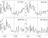
Figure 3 depicts the daily averaged amplitudes of oscillations measured by the ionosonde for a period from January 1 to February 28. Four bands from the shortest (10–15 min) to the longest (60–120 min) periods of AGW are shown. One can see that that the small and medium scale waves considerably decay after 20 January, i.e. just at the minimum of mesopause temperature, while the large scale waves are less affected. Comparison of Figure 3 and the left panel of Figure 2 shows that the reduction occurs almost simultaneously with the reversal of mesospheric wind. Thus the reduced AGW activity in the ionosphere are likely related to selective filtering of upward propagating AGWs due to westward mean flow in the MLT region. Also, the small-scale vertical inhomogeneity and turbulent processes may play a role in wave filtering and support its breaking.
 |
| Figure 4 |
The atmospheric turbulence may arise in the vertically narrow thermal inversion layer of $\sim 10$ K that is superimposed upon the normally decreasing temperatures of the upper mesosphere and occurred predominantly between 90 and 100 km in altitude [Meriwether and Gerrard, 2004]. Figure 4 displays vertical temperature profiles at the altitudes from 1 to 0.001 hPa for each of the 12 days ranging from January 17 to January 28 so that the first five days precede and the last five days follow the peak thermal perturbation (January 22–23) in the stratosphere and mesosphere. One can see that considerable thermal inversion layer is observed during the peak of SSW. The horizontal solid line marks the altitude of $\sim 90$ km (0.003 hPa). At 90 km altitude the temperature is at least 10 K greater than that before and after a SSW.
The AGW activity in the thermosphere is controlled by the selective filtering of waves traveling upward from the lower atmosphere. Since AGWs tend to propagate against mean zonal winds, the eastward mean flow filters out many of upward propagating eastward waves. During a SSW, a weakening and reversal of the stratospheric jet from eastward to westward permits eastward AGWs to penetrate into the MLT region while the westward AGWs (which are generally less active) are blocked. However, a decay of AGWs at $\sim 200$ km altitude just after the reversal of mesospheric wind cannot be explained by such filtering and another factor is needed. It can be a deepening of the inversion layer which manifests an increased turbulence in the MLT region since the topside of the inversion layer where the temperature decreases with increasing altitude may be convectively unstable. In particular, in January 22–23 the Richardson number of the critical layer is less than a threshold of 0.25, i.e., it is small enough to be a potential reason of the enhanced turbulence. It is known that minimal permissible horizontal wavelength of AGWs in the atmosphere is determined by viscosity (note that the turbulent viscosity is greater than the molecular one) and is proportional to the square root of it for the fixed wave frequency, whereas for the given viscosity the horizontal wavelength is proportional to $T^{3/2}$, where $T$ is a wave period [Gossard and Hooke, 1975]. The result that AGWs with periods 60–120 min are not affected by a deep inversion layer can be explained by the fact that these waves have larger horizontal wavelengths.
In the vicinity of the stratospheric polar night jet a pronounced sudden mesospheric cooling linked to a major mid-winter SSW is observed in 2009 under conditions of low solar activity. Mesosphere-ionosphere anomalies include the following features. Mesospheric cooling is almost of the same value as the stratospheric warming $(\sim 50$ K) but less long-lived. Deepening of the thermal inversion layer near the mesopause is observed during a peak of cooling. During the SSW a wind reversal from eastward to westward occurs in the stratosphere and mesosphere. Just after the mesospheric temperature reaches its minimum, the AGWs occurrence in the ionosphere with periods of 10–60 min decay abruptly while that with longer periods are not affected. The effect of such weakening of the mesosphere-ionosphere coupling may be explained by selective filtering and increased turbulence near the mesopause.
De Wit, R. J., R. E. Hibbins, P. J. Espy (2014), The seasonal cycle of gravity wave momentum flux and forcing in the high latitude northern hemisphere mesopause region, J. Atmos. Sol. Terr. Phys., 127, p. 21–29, doi:10.1016/j.jastp.2014.10.002.
Gossard, E., W. Hooke (1975), Waves in the Atmosphere, 456 pp., Elsevier, New York.
Kozlovsky, A., T. Turunen, T. Ulich (2013), Rapid-run ionosonde observations of traveling ionospheric disturbances in the auroral ionosphere, J. Geophys. Res. Atmos., 118, p. 5265–5276, doi:10.1002/jgra.50474.
Labitzke, K., B. Naujokat (2000), The lower Arctic stratosphere in winter since 1952, SPARC Newsletters, 15, p. 11–14.
Lukianova, R., A. Kozlovsky, S. Shalimov, T. Ulich, M. Lester (2015), Thermal and dynamical perturbations in the winter polar mesosphere–lower thermosphere region associated with sudden stratospheric warmings under conditions of low solar activity, J. Geophys. Res. Space Phys., 120, p. 5226–5240, doi:10.1002/2015JA021269.
Meriwether, J. W., A. J. Gerrard (2004), Mesosphere inversion layers and stratosphere temperature enhancements, Rev. Geophys., 42, p. RG3003, doi:10.1029/2003RG000133.
Received 14 September 2016; accepted 16 September 2016; published 21 September 2016.

Citation: Lukianova Renata (2016), Thermal and dynamic perturbations in the winter polar upper atmosphere associated with a major sudden stratospheric warming, Russ. J. Earth Sci., 16, ES4003, doi:10.2205/2016ES000575.
Copyright 2016 by the Geophysical Center RAS.