
RUSSIAN JOURNAL OF EARTH SCIENCES, VOL. 16, ES3001, doi:10.2205/2016ES000568, 2016
V. Kaftan1,2, A. Melnikov2
1Geophysical Center of the Russian Academy of Sciences, Moscow, Russia
2Agro-Technological Institute, Peoples' Friendship University of Russia, Moscow, Russia
The results of observation of Global Navigation Satellite Systems (GNSS) in areas of large earthquakes are analyzed in this article. The Earth's surface deformation characteristics before, during and after the earthquake are researched, the results indicate the presence of abnormal deformation near their epicenters. The statistical evaluation of abnormal deformations with their root mean squares (rms) are presented. Conclusions about the possibilities of using local GNSS observation networks for evaluation of risk of strong seismic events are performed.
Researches of deformation earthquake precursors were on the front burner from the middle to the end of the previous century. The repeated conventional geodetic measurements such as precise leveling [Kaftan and Ostach, 1996] and linear-angular networks have been used for the study. Many examples of studies referenced to strong seismic events using conventional geodetic techniques are presented in [Rikitake, 1976]. One of the first case studies of geodetic earthquake precursors was done by Mescherikov [1968].
Rare repetitions, insufficient densities and locations of control geodetic networks made difficult predicting future places and times of earthquakes occurring.
Intensive development of Global Navigation Satellite Systems (GNSS) during the latest decades allows doing the research in a more effective level.
Today permanent GNSS stations are being installed widely all over the world. It is possible now to study the Earth's surface deformation on a scale never possible before. Some of permanent GNSS networks are covering the seismo-generating zones. One of the more investigated seismic areas is San Andreas Fault zone of California, USA [Wallace, 1990]. Two of GNSS networks of this zone are well placed to study Earth's surface deformation just near the epicenters of the strong Parkfield (September 28, 2004, $Mw=6.0$) and El Mayor Cucapah (April 4, 2010, $Mw=7.2$) earthquakes. The epicenters of the earthquakes are conveniently located several kilometers far from the permanent GNSS networks.
|
| Figure 1 |
The Parkfield permanent GPS network of the Plate Boundary Observatory, USA, was used for the study of the Earth's surface deformation in relation to the Parkfield earthquake (Figure 1). The usage of the network for the study of seismic displacements is described in [Langbein and Bock, 2004].
 |
| Figure 2 |
The California Real Time Network (CRTN) of permanent GPS stations (Figure 2) is located not far from the epicenter of El Mayor Cucapah main shock and covers epicenters of some aftershocks of it. The Southern California Integrated GPS network is described particularly in [Hudnut et al., 2001].
The only shortest baseline vectors formed the Delauney triangulation were used in the processing as it is recommended in [Dokukin et al., 2010] and shown at Figure 1 and Figure 2.
 |
| Figure 3 |
The block flow diagram of the analysis is shown at Figure 3.
Observation data used for the deformation analysis was received from the archive of the Scripps Orbit and Permanent Array Center (SOPAC) [http://sopac.ucsd.edu/]. Data sampling is equal to 30 s. Daily measurements were processed using MAGNET Tools software for the determination of baseline vectors and its co-variation matrices. Such processing was performed for the 6 measurement epochs for both GNSS networks. Then the obtained baseline vectors were adjusted using the special technique. The two dimensional approach of the deformation analysis has been used in the study. It is recommended as a proper and unified example in [Dermanis and Kotsakis, 2005].
The procedure of the adjustment is described as follows. Observation equations were presented as
\begin{equation} \tag*{(1)} v= Adx + l \end{equation}where $v$ – vector of the derived corrections to the differences of repeatedly measured baseline components of the order $(3n-3) \times 1$ for $n$ baselines; $A$ – matrix of the coefficients of the observation equation (1); $dx$ – vector of point displacements of the order $3k \times 1$ in case of $k$ determinate points; $l$ – vector of the differences of the measured network elements of the order $(3n-3)\times 1$.
The Least Square solution of the observation equations (1) is
\begin{eqnarray*} dx = - N^+L = - Q_{dx} L \end{eqnarray*}where $N= A^T Q_l^+ A$ and $L= A^T Q_l^+ l$, the so-called matrix of the normal equations coefficients and vector of the free terms of the normal equations, where $Q_l^+=P$ is the matrix of the weights of the measurements.
This solution satisfies not only the condition $v^T Pv=\min$ but the $x^T Q_x^+ x =\min$ too.
The adjustment procedure makes possible to calculate the plan deformation characteristics. Principal deformations $\gamma_1$, $\gamma_2$ and dilatation $\Delta$ have been used in this study.
\begin{eqnarray*} \gamma_1 = [x_2(dy_3 - dy_1) + y_2(dx_3 - dx_1) - x_3(dy_2 - dy_1) - \end{eqnarray*} \begin{eqnarray*} y_3(dx_2 - dx_1)] \Big/ (x_2y_3 - x_3y_2) \end{eqnarray*} \begin{eqnarray*} \gamma_2 = [x_2(dx_3 - dx_1) + y_2(dy_3 - dy_1) - x_3(dx_2 - dx_1) - \end{eqnarray*} \begin{eqnarray*} y_3(dy_2 - dy_1)] \Big/ (x_2y_3 - x_3y_2) \end{eqnarray*} \begin{eqnarray*} \Delta = [x_2(dy_3 - dy_1) - y_2(dx_3 - dx_1) - x_3(dy_2 - dy_1) + \end{eqnarray*} \begin{eqnarray*} y_3(dx_2 - dx_1)] \Big/ (x_2y_3 - x_3y_2) \end{eqnarray*}where $x_i$, $y_i$ are plan coordinates; $dx_i$, $dy_i$ – plan displacements; $i$ – indices of vertex of triangles.
 |
| Figure 4 |
 |
| Figure 5 |
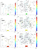
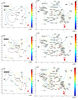
Displacements and deformations were calculated for the three epoch differences before and three epoch differences after the El Mayor Cucapah earthquake. Corresponding characteristics referenced to the Parkfield earthquake were received from the study [Kaftan et al., 2010]. The plan displacement vectors and vertical displacement isolines are presented in Figure 4 and Figure 5. The visual comparison of these characteristics does not allow to see some abnormal earth surface behavior before the earthquakes.
 |
| Figure 6 |
 |
| Figure 7 |
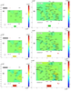
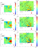
The graphical contour maps of the dilatation patterns and the main strain axes as a result of the "quick look" analysis are presented in Figure 6 and Figure 7 in comparison to each other. Figure 6 shows the existence of substantial Earth's surface deformations prior to the both earthquakes rising in time approaching to the moments of the main shocks. The main extremes of deformations are placed near the earthquake epicenters. It is possible to consider that these features have to be considered as the earthquake precursors. The postseismic deformations are shown at Figure 7. It accelerates in the same locations in relation to the preseismic patterns.
 |
| Table 1 |
The quantitative estimates of the dilatation $\Delta$ and root mean square errors $\sigma_\Delta$ of every observation interval for both study cases are represented in the Table 1. Preseismic and postseismic dilatation values are written in the top and bottom parts of the Table 1 respectively. The values of preseismic deformations vary from 0.1 to $1.8 \times 10^{-5}$. The world practice demonstrates that so high level of deformation corresponds to seismic processes. These values of deformations can be considered as alarms of approaching to seismic event occurrences near its localizations.
In the case of the adopted adjustment technique it is possible to test the general statistical efficiency of displacement vectors determination. For this purpose we compute the ratio [Kaftan, 2003]
\begin{eqnarray*} F=\frac{dx^T N dx}{v^T Pv} \end{eqnarray*} |
| Table 2 |
and set a confidence level $\alpha$ according to a freedom degree $n-k$ with the use of $F$-distribution tables setting up the critical value $F_{(\alpha,n-k,n-k)}$. The results of the testing are shown in Table 2.
As it is seen from the Table 2 all $F$ ratios confidently exceed the critical values. It attests to the presumption that the level of displacements is much higher than the level of the measurement accuracy.
The range of extremal dilatation values $R_\Delta=\Delta_{\max} - \Delta_{\min}$ was used as other criterion of the abnormal deformation of the studied territory. It presented in the Table 2. It is possible to consider that the range values can be thought of as deformation precursors of the strong earthquake occurrence.
Two studied cases of horizontal deformation behavior before and after strong earthquakes show the contrast deformation changes from years by days before the events near their epicenters.
The estimated extremes can be considered as temporal precursors of the earthquake occurring.
It is possible that the places of the earthquake occurring can be predicted using the extremes too.
The permanent GNSS networks covering seismic generating fault zones can be effective tools for the earthquake prediction.
The further research will be continued to reveal the more detailed tendencies and regularities of Earth's surface deformation behavior in seismo-generating zones.
Dermanis, A., Ch. Kotsakis (2005), Estimating Crustal Deformation Parameters from Geodetic Data: Review of Existing Methodologies. Open Problems and New Challenges, International Association of Geodesy Symposia, 131, p. 7–18.
Dokukin, P. A., V. I. Kaftan, R. I. Krasnoperov (2010), The influence of the form of triangles in geodetic network on determining of Earth's surface deformation, Proceedings of the Univers. Geodesy and Aerophotosurveying, 5, p. 6–11 (in Russian).
Hudnut, K. W., et al. (2001), The Southern California Integrated GPS Network, Proceedings of the 10th FIG International Symposium on Deformation Measurements, 19–22 March 2001, p. 129–148, Orange, California, USA.
Kaftan, V. I. (2003), Temporal analysis of geospatial data: Kinematic models, Thesis for a doctor's degree, Moscow State University of Transportation, Moscow (in Russian).
Kaftan, V. I., O. M. Ostach (1996), Vertical land deformation in Caucasus region, Earthquake Prediction Research, 5, p. 235–245.
Kaftan, V. I., R. I. Krasnoperov, P. P. Yurowsky (2010), Gra-phical representation of results of the earth's surface movements and deformations determination by means of global navigation satellite systems, Geodesy and Cartography, no. 11, p. 2–7 (in Russian).
Langbein, J., Y. Bock (2004), High-rate real-time GPS network at Parkfield: Utility for detecting fault slip and seismic displacements, Geophysical Research Letters, 31, p. L15S20, doi:10.1029/2003gl019408.
Mescherikov, J. A. (1968), Resent crustal movements in seismic regions: Geodetic and geomorphic data, Tectonophysics, 6, p. 29, doi:10.1016/0040-1951(68)90024-3.
Rikitake, T. (1976), Earthquake Prediction, 357 pp., Elsevier, New York.
Wallace, R. E. (ed.) (1990), The San Andreas fault system, California. U.S. Geological Survey professional paper 1515, 405 pp., Government Printing Office, Washington, D.C., U.S.
Received 8 August 2016; accepted 20 August 2016; published 27 August 2016.

Citation: Kaftan V., A. Melnikov (2016), Deformation precursors of large earthquakes derived from long term GNSS observation data, Russ. J. Earth Sci., 16, ES3001, doi:10.2205/2016ES000568.
Copyright 2016 by the Geophysical Center RAS.