Methods

[9]  To obtain the results given in the paper we used four major methods to study observation series.

Method 1. Revealing Asymmetric Impulses

[11]  The operations to calculate and to remove trends are as follows. Let X(t) be arbitrary limited integrated signal with continuous time. Let kernel averaging with scale parameter H>0 be called the average value of X (t|H) in the time moment t calculated by formula:

(1)

where y(x) is arbitrary non-negative limited symmetric integrated function called averaging kernel [Hardle, 1989]. If y(x) = exp (- x²), value is called Gaussian trend with parameter (radius) of averaging H [Hardle, 1989; Lyubushin, 2007].

[12]  As a result of the above-described preliminary operations we obtain a signal with discretization interval of 1 sec with power spectrum in the period range approximately from 3 to 30 minutes The same result can be obtained with the common band Fourier filtration but Gaussian trends are more preferable because side effects caused by filter discrimination are missing and besides it is easier to control boundary effects caused by the finite character of the sampling being filtered.

[13]  To analyze impulse sequence in the quantitative sense a program was developed to separate them automatically. We used Haar expansion by wavelets [Daubechies, 1992; Mallat, 1998]. After direct Haar wavelet transformation only a small part (1- a ) of wavelet coefficients maximal in magnitude was left with a = 0.9995. Then reverse wavelet transformation was performed and as a result a sequence of impulses was separated with large amplitudes divided from one another with intervals of constant values that had been filled with noise before. In wavelet analysis, this operation is known as denoising [Daubechies, 1992; Mallat, 1998]. Haar wavelet was chosen for this operation because of simplicity of subsequent automated separation of rectangular impulses. The number of separated impulses and the extent of noise rejecting depend on the selected compression level a.

Method 2. Detecting Periodic Components in the Sequence of Events

(2)

where frequency w, amplitude a, 0 a 1, phase angle j, j [0, 2p] and factor m 0 (describing Poisson part of intensity) are the model parameters. Thus Poisson part of intensity is modeled by harmonic oscillations.

[15]  Owing to considering an intensity model richer than for a random series of events and with harmonic component of given frequency w, the likelihood logarithmic function increment of point process [Cox and Lewis, 1966] is equal to [Lyubushin et al., 1998]:

(3)

Here t_i is the sequence of time moments of separated local maximums of the signal inside the window; N is the number of them; T is the length of time window. Suppose

(4)

[16]  Function (4) may be considered as spectrum generalization to the sequence of events [Lyubushin et al., 1998]. The plot of the function shows how much more favorable the periodic model of intensity is as compared to a purely random model. Maximum values of function (4) indicate frequencies present in the event sequence.

[17]  Let t be the time of the right edge of the moving time window of preset length T_W. Expression (4) is actually a function of two arguments: R (w, t | T_W), which can be visualized in the form of 2-D map or 3-D relief on the plane of arguments (w, t). This frequency-time diagram allows us to study the dynamics of appearance and development of periodic components inside the event flow under investigation [Lyubushin, 2007; Sobolev, 2003, 2004; Sobolev et al., 2005].

Method 3. Initial Data Transformation Into Variations of Hurst Generalized Exponents

[19]  Note that the analysis of multifractal characteristics of geophysical monitoring time series is one of promising lines of data studies in the solid earth physics. [Currenti et al., 2005; Lyubushin, 2007; Telesca et al., 2005]. It is determined by the fact that multifractal analysis is capable of investigating signals that are nothing more than white noise or Brownian motion in terms of covariation and spectrum theory.

[20]  Let X (t) be a signal. We define the amplitude as variation measure m (t, d) of the signal behavior X (t) at interval [t, t + d]:

(5)

[21]  Holder-Lipschitz index h (t) for point t is defined as limit:

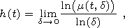(6)

that is in the vicinity of point t signal variation measure m (t, d) with d 0 descents by law d^h(t).

[22]  Singularity spectrum F(a) is defined [Feder, 1989] as fractal dimensionality of a set of points t, for which h(t)=a (that is having the same Holder-Lipschitz index equal to a ).

[23]  The existence of singularity spectrum is ensured not for all signals but only for the so-called scale-invariant ones. If X(t) is a random process, let us calculate the average value of measures m(t, d) in exponent q:

(7)

[24]  Random process is called scale-invariant if M(d, q) with d 0 descents by law d^k(q), that is to say the limit exists:

(8)

[25]  If the dependence k(q) is linear: k(q)=Hq, where H= const, 0H=0.5. Process X(t) is multifractal if dependence k(q) is non-linear.

[26]  The idea of raising to different powers q in formula (7) implies that different weights may be given to time intervals with big and small measures of signal variability. If q>0, then the major contribution into the average value M(d, q) is made by time intervals with great variability, whereas time intervals with small variability make maximum contribution with q<0.

[27]  If we estimate spectrum F(a) in moving time window its evolution may give information on the variation of the series random pulsations. Specifically the position and width of the spectrum carrier F(a) (values a _min, a _max and Da=a _max-a _min and a are given to function F(a) by maximum: F(a)= max_a F(a)) are noise characteristics. Value a can be called generalized Hurst exponent. For monofractal signal the value of Da is to be equal to zero, and a=H. As for the value of F(a), it is equal to fractal dimensionality of points in the vicinity of which scaling relationship (8) is fulfilled.

[28]  Below to calculate singularity spectrum F(a) we applied the detrended fluctuation analysis [Kantelhardt et al., 2002] in programs given in detail in [Lyubushin, 2007; Lyubushin and Sobolev, 2006].

[29]  Commonly F(a)=1, but in some windows we found F(a)<1. Recall that in the general case (not only for time series analysis) value F(a) is equal to fractal dimensionality of multifractal measure support [Feder, 1989].

Method 4. Calculations of Spectral Measure of Coherence

[31]  Spectral measure of coherence l(t, w) is built as modulus of the product of canonical coherence component by component.

(9)

[32]  Where q is the total number of time series analyzed together (dimensionality of multidimensional time series); w is frequency; t is time coordinate of the right edge of the moving time window comprising a certain amount of adjoining points; n_j(t, w) is canonical coherence of j -scalar time series, which describes the strength of coherence between this series and all other series. Value | n_j(t, w)|² is generalization of common square spectrum of coherence between two signals when the second signal is not scalar, but vector. Inequality 0 | n_j (t, w) | 1 is fulfilled and the closer is value | n_j (t, w)| to one, the stronger are linearly connected variations at frequency w in time window with coordinate t of j -series with analogous variations in all other series. Correspondingly value 0 l (t, w) 1 owing to its construction describes the effect of cumulative (synchronous, collective) behavior of all the signals.

[33]  Note that, from the construction, the value of l(t, w) belongs to interval [0,1], and the closer are corresponding values to one the stronger is the connection between variations of the multidimensional time series components Z(t) at frequency w for time window with coordinate t. It should be emphasized that comparing absolute values of statistics l(t, w) is only possible for one and the same number q of time series processed simultaneously since by formula (9) with the increase of q value l decreases, being product of q values that are below one.

[34]  To implement this algorithm the spectral matrix assessment of the initial multidimensional series is required in each time window. In the following, preference is given to the use of vector autoregressive model of the 3rd order [Marple, 1987]. We took time window length equal to 109 values to obtain relationship l(t, w). Since each value of a was obtained from time window of a length of 12 hours and the shift of those windows is 1 hour, then the length of time window to assess the spectral matrix is (109-1) 1+12 = 120 hours = 5 days.

Powered by TeXWeb (Win32, v.2.0).