4. Relation between Various Types of Remanent Magnetization

Figure 2

[38]  Thus, comparison of thermoremanent ( I_rt ) and anhysteretic ( I_ri ) magnetizations in ensembles of single-domain particles coinciding (narrow spectrum) and differing (wide spectrum) in coercivity [Afremov and Kharitonsky, 1986a, 1986b] shows that R_t = I_rt/I_ri < 1 for a system of weakly interacting grains and R_t > 2 for strongly interacting grains (Figure 2). The dependence of the ratio between chemical and anhysteretic magnetization R_c = I_rc/I_ri on the factor F defined by Sholpo [1977]

Figure 3

is plotted in Figure 3. The curves R_c = R_c(F) are similar in behavior to R_t = R_t(B), which is quite natural because F B/H _max at F1.

[39]  Comparing R_t and R_c, it is easy to show that, with increasing H_{c max}, the parameter R_c reaches an ultimate value at greater values of B than the parameter R_t does. This is due to the fact that the chemical and thermoremanent magnetizations are mainly due to, respectively, low- and high- coercivity grains. Note also that, in the experimentally observed range of interaction fields ( B 3-30 Oe) [Ivanov et al., 1981; Ivanov and Sholpo, 1982], the maximum value of R_c is R_c 1, whereas R_t depends on coercivity.

[40]  Knowing the response of each particle to an external effect (variations in H_c and I_s and the corresponding displacements of representative points in a diagram), we can easily calculate all of the aforementioned types of remanent magnetization and establish the relations between them.

[41]  The function g(|H|) can also be applied for the estimation of detrital magnetization in a system of large particles whose orientation is modified by a magnetic interaction field rather than temperature. This estimate is directly related to the so-called cluster model of depositional magnetization developed in [Shashkanov et al., 1989, 2003

[42]  Using the distribution density given by (4), one can show [Belokon and Nefedev, 2001] that, before the decrease in the tilt angle of a certain portion P of elongated or flattened particles, the detrital magnetization is given by the formula

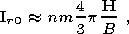(26)

where H is the external field. After the particles become less tilted, we have

(27)

(28)

Here (p2- ₀) is the inclination of I_r0 and ₀-₀ is its error.

[43]  In conclusion, we can note the following.

[44]  (1) Knowledge of values of R_t and R_c is insufficient for the identification of thermoremanent and chemical magnetizations in an ensemble of single-domain particles. This identification requires additional information on the coercivity and the intensity of magnetostatic grain interaction that can be obtained from laboratory experiments.

[45]  (2) Spontaneous magnetization can change with time due to diffusion processes [Afremov and Belokon, 1972]. This can lead to stabilization of the vector I_s and a rise in the magnetic moment of the system (diffusion-induced viscous magnetization).

[46]  (3) The formation of chemical magnetization can be interpreted in terms of a mechanism [Belokon et al., 1995] that is an analogue of the thermoremanent magnetization formation mechanism and differs from the crystallization mechanism proposed by Haig [1962].

Powered by TeXWeb (Win32, v.2.0).