RUSSIAN JOURNAL OF EARTH SCIENCES, VOL. 20, ES4007, doi:10.2205/2020ES000735, 2020

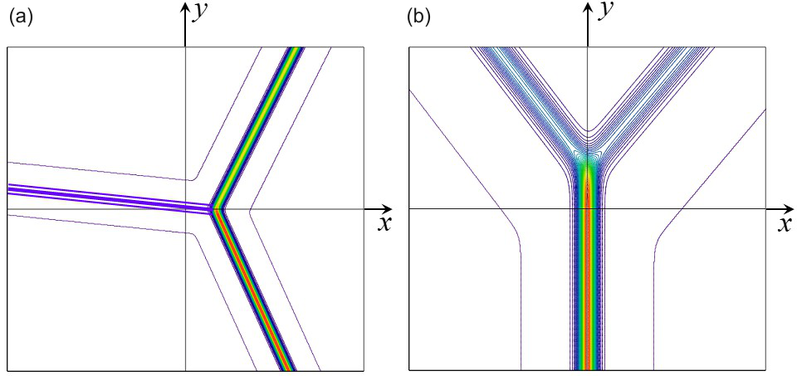
Figure 5. (colour online). Contour-plots of soliton fronts as per solution (12), (13) and (5) with the soliton parameters are: $k_{1} = 1$, $k_{2} = 1.1$, $l_{2} = -l_{1}$, soliton amplitudes are $A_{1} = 3$, $A_{2} = 3.63$. In frame (a) $l_{2} = l_{c1} = 9.072647087265 \times 10^{-2}$ so that $B = 0$; in frame (b) $l_{2} = l_{c2} = 1.90525588833\times 10^{-2}$ so that $B = \infty$. The plot was generated for $\alpha = \beta = 1$ and $c = 2$ in the domain $(-100, 100) \times (-500, 500)$ in frame (a) and in the domain $(-250, 250) \times (-1000, 1000)$ in frame (b).

 
Citation: Ostrovsky L. A., Y. A. Stepanyants (2020), Kinematics of interacting solitons in two-dimensional space, Russ. J. Earth Sci., 20, ES4007, doi:10.2205/2020ES000735.
 

Copyright 2020 by the Geophysical Center RAS.