Thermomechanics of phase transitions of the first order in solids

V. I. Kondaurov

Moscow Institute of Physics and Technology, Moscow, Russia

Contents

Abstract

A generalized Clapeyron-Clausius equation governing the differential dependence of the phase transition temperature on the initial phase deformation is formulated. The paper presents a new relation of the phase transformation theory, namely, the equation describing the differential dependence of the phase transition temperature on the interface orientation relative to the anisotropy axes and the principal axes of the initial phase strain tensor. Based on the relations derived in this study, the phase transformation temperature of an initially isotropic material is shown to assume extreme values if the normal to the interface coincides with the direction of a principal axis of the initial phase strain tensor. The phase transition of the first order in a linear thermoelastic material with small strain values and small deviations of the temperature from its initial value is discussed in detail. A class of materials is distinguished in which an increase in the initial phase strain necessarily changes the character of the phase transformation (a normal phase transition becomes an anomalous one and vice versa). The equilibrium of a compressed viscoelastic layer admitting melting and the effect of stress relaxation in the solid phase on the fluid boundary motion are examined.

1. Introduction

As is experimentally shown, nearly all materials experience phase transitions under sufficiently intense thermal and mechanical loads. Two cases can be distinguished depending on properties of the phase material. In the first case, new phase nuclei unboundedly grow and coalesce, finally forming large regions each consisting of only one phase. The contact surface of such a region, below referred to as an interface, is a surface at which some thermodynamic parameters and their first derivatives are discontinuous. One of the main problems of the phenomenological theory of such transitions is to specify the relations between various quantities at the interface. In the second case, energy factors and kinetic properties restrict the growth of new phase nuclei by medium-scale sizes that are small compared to the characteristic size of a body. The accumulation of nuclei that do not coalesce gives rise to a mixture of two phases and a composite structure consisting of an initial phase matrix "reinforced" by inclusions of the new phase disseminated throughout its volume. In this case, in addition to the problem of determining the effective properties of this type of materials, which is traditional in the mechanics of composites, one often encounters the problem the phenomenological description of the concentration, spatial distribution and shape of the new phase inclusions as a function of varying stress (strain) and thermal state. In this study I restrict myself to the first case (below referred to as the phase transition of the first order in accordance with the generally accepted terminology).

The majority of natural processes are associated with or even due to phase transformations of materials [Turcott and Schubert, 1982], and many of these processes are critically dependent on not only the temperature and pressure but also tangential stresses. Examples are tectonic processes, metamorphism phenomena, stratification in the crust and recrystallization of geomaterials. The formation of deep-seated sources of earthquakes is associated with the relaxation of deviatoric stresses in the vicinity of a moving front of phase transformations. The orientation and shape of magma chambers essentially depend on the presence of shear stresses and thermoelastic properties of the surrounding rocks. The list of geophysical examples alone can be continued. However, even the aforesaid clearly indicates the relevance of the correct description of the problem of solid phase transformations.

Mechanics and thermodynamics of phase transformations of deformable solids have been developed over more than a century [Gibbs, 1906]. The theory of liquid and gas phase equilibrium reducing to the equality of pressures, temperatures and chemical potentials has become a constituent of the classical thermodynamics and statistical mechanics [Landau and Lifshits, 1964] and a working tool in solving many scientific, engineering and technological problems [Christian, 1978; Khachaturyan, 1974; Roitburd, 1974]. On the other hand, the Gibbs approach to the description of the phase equilibrium conditions brought about many studies intended to extend this approach to deformable solids in a nonhydrostatic stress state and to the construction of the scalar chemical potential in media characterized by more than two scalar parameters of state. Such studies are reviewed, for example, in [Grinfeld, 1990; Ostapenko, 1977], where these problems are also discussed in detail. Investigations in this direction continue presently as well [Knyazeva, 1999].

The first question arising in phenomenological simulation of phase transformations is the following: How can the first-order phase transition be defined in terms of the continuum mechanics? In the existing literature, this question is either ignored or the phase transition is treated as a change in the aggregate state of a solid, which is simply a paraphrase reducing to the replacement of one term by another, equally indefinite term. Some authors invoke to the structure of the medium and to the size and other characteristics of the solid lattice, i.e. to the notions beyond the system of concepts of continuum mechanics and thermodynamics. Phases are, at best, defined as states of the matter coexisting as macroscopic regions that are at equilibrium with each other and are separated by surfaces at which some thermodynamic potentials are discontinuous [Landau and Lifshits, 1964]. Setting aside insignificant, in my opinion, limitations inherent in a purely static case, this definition implicitly refers to the main problem related to the loss of uniqueness of the response of the medium to a given thermodynamic state. In what follows, remaining within the framework of thermodynamics of irreversible processes, phase transitions of the first order in a continuum will be understood as processes associated with the transition of a material element from one branch of the response functional or function to another. The main problem in the theory of first-order phase transitions is the thermodynamic conditions consistent with such a transition; the latter can be either slow or rapid (dynamic) transition. As distinct from the traditional approach based on variational principles, this work describes the first-order phase transitions in deformable solids within the framework of the theory of strong discontinuities in the solution of partial differential equations describing the behavior of the continuum studied. The necessary condition for constructing a closed system of equations involving strong discontinuities is the possibility of representing the equations as a system of conservation laws, which means that these equations can be written in a divergent form. Hence, the first-order phase transition in materials of the Prandtl-Reuss elastic-plastic type of the medium [Sedov, 1970], equations of which are basically irreducible to a divergent form in the case of a multidimensional strain state, cannot be described in terms of the conventional approach and require the application of the general theory of strong discontinuities [Sadovskii, 1997].

From the standpoint of the approach adopted in this study, the phase transition can be realized not only in materials described by a general equation of state of the Van der Waals type whose nonconvexity ensures the nonuniqueness of the material response to a given state. As is shown below, phase transformations can be experienced by materials the responses of which are described by different, completely independent equations of state of each of the phases present. Moreover, each of these constitutive equations can satisfy the convexity condition and other classical restraints imposed on thermodynamic potentials.

Note also that, in constructing the so-called wide-range equations of state with high densities of energy, the plane of state variables is often subdivided into fields of different states of phases [Bushman et al., 1992; Melosh, 1989]. Such a subdivision is an approximate approach because the localization of various phase fields ignores the solid-state properties of the material, the loading rate dependence of the phase equilibrium conditions and the possible overlapping of the areas of phase existence. Such an approximation cannot be substantiated by a local thermodynamic equilibrium of the material element. A characteristic example is the distinction of the Hugoniot adiabat describing the behavior of a material under a shock load from the isotherm corresponding to a slowly varying mechanical and thermal load.

The quasi-thermostatic approximation is often applied to the modeling of first-order phase transitions caused by slowly varying mechanical and thermal loads. This approximation implies that the state of a material element is supposed to be close to a thermomechanical equilibrium characterized by a temperature gradient qq₀/l₀ and an Euler number r₀v²₀/s₀1, where q₀, l₀, r₀, v₀ and s₀ are the characteristic temperature, linear size of the body, density, velocity and pressure, respectively. It is additionally assumed that the velocity of the interface is small compared to the velocity of sound, and no singular sources of mass, momentum, energy and entropy are present on the interface.

The assumption of the smallness of temperature gradients means that the model used precludes temperature discontinuities, because otherwise the temperature gradient between two points on opposite sides of the discontinuity surface will be infinitely large. The quasi-static approach implies that the inertia forces and kinetic energy are neglected in the equations of motion and energy balance, respectively. The absence of a singular source of entropy means that the phase transition in such a material is a reversible process for which the Clausius-Duhem inequality becomes an equality. Hence, dissipation vanishes not only in smooth flow areas but also as a particle crosses the interface. The phase transition reversibility assumption is less evident and is often used implicitly, particularly if phase transitions are described in terms of variational principles of the continuum mechanics [Grinfeld, 1990].

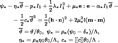
2. Basic Relations of a Thermoelastic Medium

Before deriving relations on a strong discontinuity surface separating different solid phases, I remind the reader of the basic definitions and formulas of the theory thermoelastic solids. The state of a material point X of a thermoelastic medium at a time moment t is specified by the set of quantities

where F is the gradient of the mapping kc(t) of the reference configuration of the body k into the current configuration c(t). The nonsymmetric second-rank tensor F connects the radius-vectors differentials of two neighboring material points:

where ⁰ is the gradient in the Lagrangian (substantial) variables Xk. The following polar decomposition holds for the nonsingular tensor F:

(2.1)

where R is an orthogonal tensor characterizing a rigid rotation of the material element as a whole, and U and V are symmetrical, positively definite tensors describing the deformation of this element.

The current response of the material point X of a thermoelastic material at the time moment t is characterized by the set of quantities

where T is the symmetrical Cauchy tensor of stresses, q is the heat flux vector, h is the entropy density and y is the free energy density connected with the internal energy density through the relation y = u - qh. The scalar q is the absolute temperature, gq is the temperature gradient and is the gradient in Eulerian (spatial) variables x c (t). In a thermoelastic material, the current response S ( X, t) is supposedly a function of the current state l( X, t), i.e.

(2.2)

where S⁺_k { T⁺, y⁺, h⁺, q⁺} is a set of functions that effect the mapping l( X, t)S( X, t) and specify mechanical and thermal properties of the material. Below, these functions are referred to as constitutive functions or relations. The index k indicates the dependence of the constitutive mappings on the choice of the reference configuration of the body.

The thermoelastic materials under consideration include both liquids and solids. In the particular case q = const, corresponding to the isothermal approximation, the constitutive relations are transformed into the model of a hyperelastic material; if undeformable heat-conductive solids are considered ( F is an orthogonal tensor in any motion), the thermoelastic model reduces to the traditional theory of heat conduction.

A necessary and sufficient condition for the validity of the second law of thermodynamics (Clausius-Duhem inequality)

in any smooth process of state variation is given by the following restraints on the constitutive relations of the thermoelastic medium [Truesdell, 1972]:

(2.3)

(2.4)

(2.5)

Relations (2.3) and (2.4) mean that, first, the free energy density of the thermoelastic medium is independent of the temperature gradient; this is not an assumption but a statement proven on the basis of general assumptions of the continuum mechanics. Second, the stress tensor and entropy density of the thermoelastic material are fully determined by the partial derivatives of a function of the free energy. Equation (2.5) implies that, in any state of the thermoelastic solid, the heat flux vector q cannot make an obtuse angle with the temperature gradient q.

The internal dissipation

in the thermoelastic material is written as

Henceforward a colon in formulas means a double scalar product such that A: B = A_ijB^ij. On the strength of (2.3) and (2.4), this yields, i.e. the thermoelastic medium is a perfect material in the sense that any smooth deformation process is not accompanied by internal dissipation. This only true of smooth flows. If a particle crosses a strong discontinuity surface, its entropy can undergo a jump at the shock wave due to the action of singular sources of entropy on the wave surface [Landau and Lifshits, 1988].

The requirement of the material independence of the reference system choice (the objectivity principle) leads to the following restraints on the constitutive equations of a thermoelastic material:

(2.6)

where R and U are the tensors in polar decomposition (2.1). I emphasize that relations (2.6) hold in a medium of an arbitrary type of symmetry.

A solid, initially isotropic thermoelastic material is particularly important in applications. The constitutive relations of such a material, written through kinematic quantities measured from the undistorted configuration of the body k₀, are invariant under the group of proper orthogonal transformations of this configuration. The free energy y⁺ ( U, q) and the heat flux vector q⁺ ( U, q, R^T q) in such a material are isotropic functions obeying the identities

where K is any orthogonal tensor with a positive determinant. Then, the constitutive equations of a solid, initially isotropic thermoelastic material can be written in the form

(2.7)

where B = F F^T = V² is the symmetrical, positively definite tensor of finite strain, and I_k ( B), k = 1, 2, 3, are principal invariants of B determined by the formulas

(2.8)

The scalar coefficients b_i = b_i (I_k, q), i = 0, 1, 2; k = 1, 2, 3 in the polynomial representation of the Cauchy stress tensor T are functions of temperature and invariants of the strain tensor B. These coefficients are completely determined by the thermodynamic potential:

(2.9)

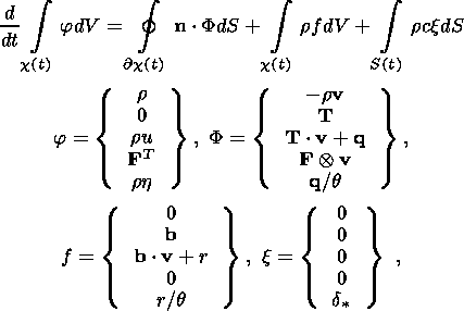
The complete system of equations of the thermoelastic material in regions of the smooth solution in the Eulerian variables (  x, t ) can be written as a system of divergent differential equations (local conservation laws):

(2.10)

(2.11)

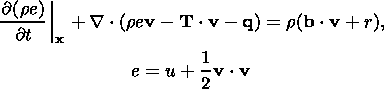(2.12)

(2.13)

Henceforward, J = det F, the symbol means the tensor product, u is the internal energy density, e = u + ¹/₂ v v is the total energy of unit mass, b is the density of body forces and r is the heat source distribution density. Relations (2.10), (2.11) and (2.12) are, respectively, equations of the local mass balance, motion and local energy balance. Equation (2.13) is a kinematic relation ensuring the compatibility of deformations and velocities of a material particle. System (2.10)-(2.13) is complemented by constitutive relations (2.6) specifying the properties of the thermoelastic material.

I should also note that the representation of a complete system of equations of a thermoelastic body through local conservation laws (2.10)-(2.13) is possible because the kinematic compatibility equation (2.13) connecting the variation rate of the tensor F with the velocity gradient of a material particle was used in conjunction with the traditional conservation laws. This equation for a nonsymmetric tensor F characterizing both the extension of a material element and its rigid rotation as a whole has a divergent form in the case of arbitrary deformations. Contrary to (2.13), kinematic relations of the type

that connect the total derivative of the Almansi finite strain tensor E = 12( I - F^-1T F^-1) (or another symmetric strain tensor) with the velocity gradient are basically irreducible to the divergent form. A more detailed discussion of this problem can be found in [Kondaurov, 1981; Kondaurov and Nikitin, 1990].

The requirement of correctness of boundary problems involving system (2.10)-(2.13), (2.6) imposes additional restraints on the free energy density y ( F, q). In the isothermal approximation, the necessary condition related to the solvability of equilibrium problems for a thermoelastic body has the form

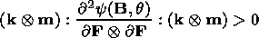(2.14)

for arbitrary vectors k 0, m 0. This inequality is called the strong ellipticity condition [Lurye, 1980; Truesdell, 1972].

In the Lagrangian (substantial) variables (  X, t ) the system of differential equations for a thermoelastic material can be written as

(2.15)

where r_k is the mass density in the reference configuration k connected with the density r in the actual configuration through the relation

(2.16)

q_k = J F^-1 q is the heat flux vector in the Lagrangian variables X, and

(2.17)

is the nonsymmetric Piola-Kirchhoff stress tensor of first kind.

3. Relations at the Interface

Here, based on the assumption that the process under study is close to the mechanical and thermal equilibrium, I discuss the conditions on the moving surface of a strong discontinuity separating two phases of a thermoelastic body experiencing finite deformations and arbitrary heating. In the general case the phases are assumed to be anisotropic solids with various types of anisotropy. Then, for each phase there exists an undistorted reference k⁽ⁿ⁾₀, n = 1, 2, such that the symmetry groups of the phase material g⁽ⁿ⁾₀ belong to a proper orthogonal group [Lurye, 1980; Truesdell, 1972]. In other words, constitutive equations (2.6) of the phase material written in terms of strains measured from the undistorted reference configurations are invariant under orthogonal transformations belonging to g⁽ⁿ⁾₀.

The configurations k⁽ⁿ⁾₀ generally differing in the density of material are interrelated via the nondegenerate transformation

where a positively definite tensor U₀ is the gradient of the nondegenerate mapping k⁽²⁾₀ k⁽¹⁾₀, and d X⁽ⁿ⁾ are the radius vectors connecting two infinitely near material particles in the configurations k⁽ⁿ⁾₀. The value U₀ interrelating undistorted reference configurations of an infinitely small material element in different phase states depends on the temperature q⁽ⁿ⁾₀ and the stress state T⁽ⁿ⁾₀ of the material in the configuration k⁽ⁿ⁾₀, i.e. U₀ = U₀ ( T⁽ⁿ⁾₀, q⁽ⁿ⁾₀). Natural configurations in which stresses vanish and the temperature q₀ is constant are most widespread in applications. The tensor U₀ is the kinematic characteristic of a phase transition in solids. In the classical theory of phase transitions, an analog of U₀ is the ratio of phase densities.

Various configurations k⁽ⁿ⁾₀ differ not only in the mass density and anisotropy properties of the material but also in its free energy and entropy. In the case of a single-phase medium, these thermodynamic potentials in the reference state are usually set equal to constants of minor importance (most often to zero). In phase transformations the difference between the free energies of phases in the configurations k⁽ⁿ⁾₀, n = 1, 2, is a fundamental value, and it is natural to call it the rheological characteristic of the first-order phase transition in solids. The same is true of the entropy density. Rheological characteristics, as well as the kinematic quantity U₀, depend on the initial temperature and initial stresses in the configurations k⁽ⁿ⁾₀.

Now I formulate the relations on the moving surface of a strong discontinuity (in crossing this surface, particles experience a phase transformation). Two of these relations are obvious, namely, the temperature continuity condition

(3.1)

and the continuity condition of the radius vector x determining the spatial position of the material particle under study at the current time moment

(3.2)

Actually, a discontinuity of the temperature q or the vector x at the moving interface necessarily leads to infinite gradients of the temperature and velocity vector arising when a particle crosses a strong discontinuity surface. This is at variance with the assumption that the conditions of the phase transformation are close to the equilibrium state.

Condition (3.2) is sometimes regarded as the definition of coherent (or martensite) phase transitions. Examples of such transitions are provided by twinning processes in crystals [Coe, 1970; Robin, 1974] and some phase transformations in iron. Some authors [Grinfeld, 1990; Truskinovskii, 1983] also discuss models of incoherent phase transformations or transitions with slip in which the normal component alone of the vector x is continuous. Incoherent transitions cannot be realized within the framework of a consistent quasi-thermostatic model with a moving phase boundary, because such a transition should be associated with an infinite values of the tangential component of the velocity vector, implying an appreciable inertia effect. Slip motions are only possible on a stationary surface which is a contact discontinuity surface not crossed by particles. Attempts at the variational description of incoherent phase transitions [Grinfeld, 1990; Truskinovskii, 1983] employ the assumption on a class of admissible variations, which is unacceptable for moving phase boundaries.

In order to derive relations for other quantities at a strong discontinuity surface, I use the material variables X X⁽¹⁾ k⁽¹⁾₀ k of the undistorted reference configuration of the body in the first phase state with the temperature q₀. This means that the deformations of the second phase are also described in terms of the initial configuration k. If the phases have the same type of symmetry, the configuration k is an undisturbed configuration for the second phase. If the phases have different types of symmetry, the material of the second phase in the configuration k should have a symmetry group defined by Noll's rule [Truesdell, 1972]. The integral balance equation in these variables has the form

(3.3)

and includes relations (2.15) written in the integral form, the strain-velocity compatibility equation, the equilibrium equation obtained from equations of motion (2.15) by ignoring its inertia term, and the entropy balance equation corresponding to the Clausius-Duhem inequality. Integral equation (3.3) accounts for the presence of a strong discontinuity surface S₀ (t) moving at a velocity c_k in the direction of the normal n_k, because this surface can contribute to the balance relation. The vectors in (3.3) are defined by the expressions

(3.4)

where x is the vector of singular sources of the d function type, with its carrier concentrated on the surface S₀ (t).

Like in the classical theory of shock waves, I assume that no singular sources of mass, momentum and energy are present on moving surfaces of strong discontinuities separating two phases. As shown below, the absence of strain incompatibility sources is ensured by continuity condition (3.2) imposed on the displacement vector. As regards a singular source of entropy d, the case d=0 corresponds, by definition, to a reversible phase transformation and the case d>0, to an irreversible phase transformation. The set of assumptions on amplitudes of these sources within the framework of the system of conservation laws is an independent part of any continuum model admitting discontinuous solutions [Kulikovskii and Sveshnikova, 1998; Sedov, 1970]. As is demonstrated by the solution of the problem on the shock wave structure in an ideal gas [Ovsyannikov, 1981; Rozhdestvenskii and Yanenko, 1978], the correctness of assumptions on the amplitudes and types of sources functioning on strong discontinuities can sometimes be demonstrated by invoking more general models in which a strong discontinuity is modeled by a region of large gradients of the solution and by passing to the model with a discontinuous solution as a limit. Apparently, such a substantiation of first-order phase transition models in solids has not been given.

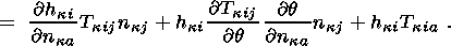
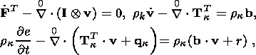
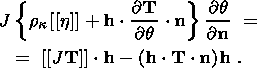
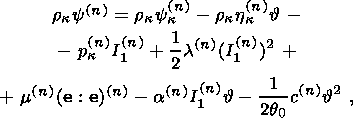
System (3.3) yields the relations for discontinuities at the phase boundary:

where [[a]] = a⁺ - a^- is the jump of a quantity a at the strong discontinuity surface, and its element under consideration is characterized by the normal n_k and by the velocity along this normal c_k. Using expressions (3.4), these relations are written as,

(3.5)

(3.6)

(3.7)

(3.8)

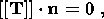
Relation (3.5) is the continuity condition of the stress vector at the phase boundary and is an analogue of the pressure continuity condition at the contact surface of liquid or gas phases. Relation (3.7) results from the continuity of the vector x( X, t) at the phase boundary and, apart from a dyadic structure of the tensor [[ F]], indicates the absence of a singular source of incompatible strains and velocities. Actually, condition (3.2) ensures the continuity of the vector d x, which is an image of the substantial vector d X S₀, i.e. [[d x]] = [[ F]] d X = 0. Since d X is arbitrary, this yields

(3.9)

On the other hand, let x be a point of a strong discontinuity surface moving at a velocity c_k in the direction of the normal n_k. Then, X/ t|_x = c_k n_k and the continuity of x = x ( X (x, t), t) yields

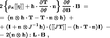
Using (3.9), I obtain

(3.10)

As seen from (3.9), the tensor [[ F]] is a dyad, and the equality (3.7) follows from (3.9) and (3.10). Using (3.10) and the relation [[ab]] = a [[b]] + [[a]] b , where a = 12 (a⁺ + a^-), energy equation (3.6) can be written in the form

Based on the continuity of the stress vector, this expression is transformed into the following:

(3.11)

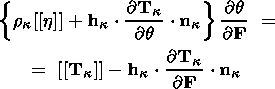
Equation (3.8) yields the normal component of the heat flux vector

substituting this expression into (3.11) and using the formula y = u - qh and the temperature continuity condition at the interface, I obtain

(3.12)

Equation (3.12) shows that the free energy density jump associated with the phase transformation of a thermoelastic material is equal to the sum of the dissipation d and the work of the stress vector r_k^-1 h_k T_k n_k on the strong discontinuity considered. Scalar equality (3.12) is an analogue of the equality condition of chemical potentials in the classical theory of the phase equilibrium of a perfect liquid (gas) [Gibbs, 1906; Landau and Lifshits, 1964]; however, they basically differ from each other because (3.12) is a continuity condition imposed on the normal components of the chemical potential tensor:

(3.13)

The equivalence of (3.12) and (3.13) can easily be shown taking into account the formula

resulting from the definition of the h_k value and the relation

In relation to reversible phase transformations ( d = 0 ), the tensor c_k was considered in works [Bowen, 1964; Grinfeld, 1990; Kondaurov and Nikitin, 1983; Mukhamediev, 1990; Truskinovskii, 1983] and is called the Lagrangian tensor of the chemical potential. The integral mass balance relation in the Eulerian variables has the form

(3.14)

and includes integral continuity equation (2.10), the equilibrium equation ensuing from equation of motion (2.11), energy conservation law (2.12) in which the kinetic energy is ignored, strain-velocity compatibility equation (2.13), and the entropy rate equation. Here S(t) is the interface moving at the velocity c = D - v n relative to material particles, D is the velocity of S(t) relative to the reference system and n is the normal to the moving interface in a current configuration. 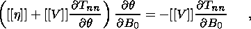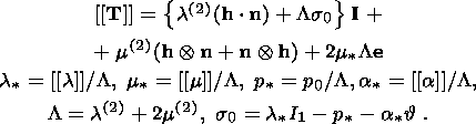Equation (3.14) yields the system of relations for jumps at a strong discontinuity surface

In the developed form, this system is written as

(3.15)

(3.16)

(3.17)

(3.18)

(3.19)

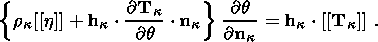
Relation (3.15) is a consequence of the continuity equation and represents the continuity condition of the mass flux. Equality (3.16), resulting from the equilibrium equation, is the continuity condition imposed on the stress vector and written in terms of the symmetrical Cauchy stress tensor.

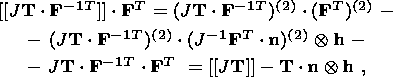
The Piola identity [Lurye, 1980] yields

providing

(3.20)

on the strong discontinuity surface. Equation (3.18) can be written in the form

(3.21)

Taking into account the continuity of the stress vector and expression (3.21) for the strain gradient jump, equality (3.17) is reduced to the form

(3.22)

Expressing with the help of (3.19) the jump in the normal component of the heat flux vector through the entropy jump and the dissipation density d and substituting the result into (3.22), one obtains equation the equality equivalent to (3.12)

(3.23)

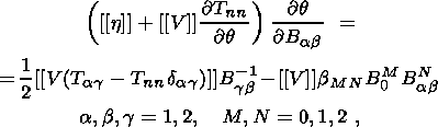
Equation (3.23) can also be written in terms of the convolution of a second-rank tensor with the normals n. To demonstrate this, I multiply (3.23) by the scalar

which is, due to (3.20), continuous at the strong discontinuity surface. As a result, I obtain

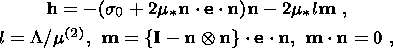
Taking into account the definition of the vector h in (3.21) implying that

the equality

(3.24)

is obtained for normal components of the tensor c, which may be called the tensor of Eulerian chemical potential. Using formula (2.17) it is easy to obtain the relation between the tensors c and c_k

demonstrating the equivalence of the spatial (Eulerian) and substantial (Lagrangian) descriptions of phase transitions in nonlinear elastic media.

Note that the dissipation d entering in conditions (3.12) and (3.23) and accounting for the effect of a singular entropy source on the interface provides a means for a natural description of the hysteresis phenomenon associated with the difference between thermodynamic conditions at which direct and reverse phase transitions of the first order take place in solids. Relation (3.12) yields

where q_d and q_r are the temperatures of direct and reverse phase transitions, and y⁽¹⁾ and y⁽²⁾ are free energies of the first and second phases. Adding these two equalities shows that q_d>q_r if y⁽²⁾ (q) in the temperature interval considered increases more rapidly than y⁽¹⁾ (q).

A recrystallization process plays a particular role among phase transitions in solids. This phenomenon relates to anisotropic solids and is a particular case of a phase transition when the initial and newly formed phases consist of the same material whose particles, when crossing the interface, undergo a finite deformation and a finite rotation changing the spatial orientation of anisotropy axes. Some authors [Grinfeld, 1990] define recrystallization as "a process changing all of the nearest neighbors of material particles," implying that the mapping of the reference configuration onto the actual configuration is no longer a one-to-one mapping. As before, in this case attempts to analyze incoherent phase transitions in terms of the quasi-thermostatic model of a thermodynamic body encounter the problem of high tangential accelerations of a material particle arising when it crosses a moving interface on which slip motions changing neighbors take place. In my opinion. such a definition is hardly suitable for the formulation and analysis of problems involving movable phase boundaries.

I should note that the requirement of a finite deformation accompanying a finite rotation of particles is essential for the recrystallization definition used here. Actually, let rotations of particles be finite and let deformations be small, i.e. the tensor F has the form

where e_k is a tensor of small strain of the order of O(d) with a small parameter d 1, and R is an orthogonal tensor of finite rotation. Then, accurate to the terms O(d²), the value B is determined by the expression

where e = R e_k R^T is the strain tensor of the order O(d). Using relation (3.21) for the strain gradient jump and the formula [[ab]] = a [[b]] + [[a]] b + [[a]] [[b]], I obtain

Taking into account that J = det F = 1 + I₁ ( e) + O (d²), F F^T = I + 2 e this relation can be reduced to the form

Since the left-hand side and two terms on the right of this equation are of the order O(d), the third term on the right must have the same order:

This gives the relations

The second equation has the solutions ( h n) = O (d) and ( h n) = -2 + O (d). Substituting the solution h n = O (d) into the first equation gives the value h = O(d) corresponding to a small jump in the rotation of a material element at the phase boundary. The solution ( h n) = -2 + O (d) describes a finite rotation jump, but this solution is unacceptable because formula (3.20), which is a consequence of the Piola identity, yields [[ F^T]] n = O(d) if the relation F = R U = R ( I + e_k) is taken into account. Hence, I obtain

The vector F^T n is not identically zero, because otherwise a nontrivial solution of the homogeneous nondegenerate linear system F^T n = 0, det F 0, should exist, implying that ( h n) = O(d); i.e. the theory of recrystallization is necessarily a finite strain theory.

4. Clapeyron-Clausius Equations

I consider the system of equations consisting of the condition of stress vector continuity (3.5) and free energy jump condition (3.12):

The superscript "2" indicates here values characterizing the second phase, and the first phase is not indexed for brevity. With regard for dyadic form (3.9) of the jump [[ F]] and temperature ( q ) continuity condition (3.1), this system can be written in the form

(4.1)

With given values of F and n_k, relation (4.1) can be regarded as a system of scalar and vector equations determining the temperature q and the vector h_k. Using relation (2.6), which connects the stress tensor and entropy density with the free energy function, and the formula F⁽²⁾_ij/ h_ka = d_ian_kj resulting from (3.9), the necessary condition of the solvability of such a system can be written as

This condition holds true if strong ellipticity condition (2.14) is valid for the newly formed phase and if M 0. System (4.1) implies that the temperature q of a quasi-static phase transition in a thermoelastic material is a function of the deformation of the initial phase and orientation of the interface:

This circumstance determines the basic distinction of phase transitions in a solid from those in an ideal liquid, in which the melting (evaporation) temperature depends on the pressure alone and is determined by the Clapeyron-Clausius equation [Landau and Lifshits, 1964]:

(4.2)

where Q = q [[h]] is the phase transition heat and [[V]] the jump of the specific volume V = 1/r. An analogue of (4.2) in a thermoelastic body is the equation

(4.3)

describing the differential dependence of the phase transition temperature on the initial phase strain F with a fixed normal n_k to the interface.

To derive this equation, I differentiate the first equation in (4.1) with respect to F at n_k = const. Since h_k = h_k ( F, n_k), q = q ( F, n_k), I obtain

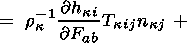
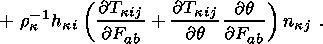
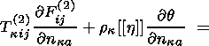
Formulas (2.6) and (2.17), stress vector continuity condition (3.5) and the formula

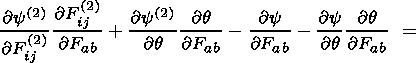
resulting from (3.9) provide the sought-for equation (4.3).

Another equation, representing a new relation in the theory of phase transformations in continua and determining the differential dependence of the phase transition temperature on the interface orientation at a fixed strain of the initial phase F, has the form

(4.4)

Relation (4.4) is obtained by differentiating the first equation in system (4.1) with respect to the vector n_k at a fixed value of the tensor F. Taking into account (2.6) and (2.17), this yields

Using condition (3.5) and the equality F⁽²⁾_ij/ n_ka = h_kid_aj + n_ka h_ki/ n_ka resulting from (3.9). The equation in question is obtained.

Equations (4.3) and (4.4) hold in a thermoelastic material with an arbitrary type of symmetry. Now I address a thermoelastic material both phases of which are initially isotropic. The kinematic characteristic of a phase transition U₀ in such a material is an isotropic tensor determined by the ratio of phase densities in natural configurations at a temperature q₀. In this case, symmetry groups of the initial and newly formed phases in the natural initial state coincide with the proper orthogonal group. The reference configurations k are undistorted for both phases; these are the natural configuration for the first phase and a configuration characterized by an initial isotropic stress tensor for the second phase. The constitutive equations can be written as relations (2.7).

Equation (4.3) containing nine independent components q/ F is reduced in the medium under consideration to a symmetrical tensor equation for the derivative q/ B, and relation (4.4) is transformed into an equation for the derivative q/ n. This statement becomes evident if one considers, rather than system (4.1), stress vector continuity condition (3.16) and energy jump relation (3.23) in the Eulerian variables:

This immediately implies that the phase transition temperature is q = q ( B, n).

In order to write equations (4.3) and (4.4) in the Eulerian variables, the following relations resulting from formulas (3.9) and (3.21) are utilized:

(4.5)

Using (4.5) and relations (2.17) between the Cauchy and Piola-Kirchhoff stress tensors, equation (4.4) can be written in the form

Taking into account formula (3.21) for a jump in the tensor F and the continuity of the stress vector, the right-hand side of this equation can be transformed as follows:

(4.6)

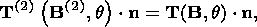
which finally yields

(4.7)

In the classical case of the phase equilibrium of an ideal liquid with the stress tensor T = -p (V, q) I, V = J/r_k = 1/r, the derivative q/ n is identically zero. Actually, due to the continuity of pressure at the interface, the right-hand side of equation (4.7) is written in this case as p( h n - [[J]]) h. This value vanishes because condition of the mass flux continuity (3.15) implies that

Taking into account the second formula in (3.21), I obtain

(4.8)

This immediately proves the above statement.

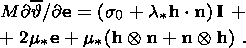
If both phases of an initially isotropic thermoelastic material are solid, an interface orientation providing an extremum of the phase transformation temperature exists at a fixed strain state of the initial phase. This extreme value is attained if one of the principal axes of the finite strain tensor B (or any other tensor coaxial with B ) coincides with the normal n to the interface. Actually, let

(4.9)

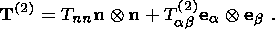
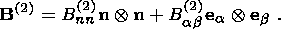
where e_a are unit vectors of the principal axes of the tensor B that lie in the plane tangent to the interface. On the strength of polynomial representation (2.7), the Cauchy stress tensor of an initially isotropic medium has the same structure:

(4.10)

As follows from the continuity of the stress vector [[ T]] n = 0, the Cauchy stress tensor has the same structure in the second phase as well:

In materials with a one-to-one correspondence between the tensors T⁽²⁾ and B⁽²⁾, this yields

Hence,

(4.11)

For the strain state under consideration, the first relation in (4.5) yields

Representing the vector h as the sum of normal and tangential components,

and substituting it into the preceding relation, I find

Comparison of this formula with (4.11) shows that h = h n, where h = r_k [[V]] = [[J]] due to (4.8). This also yields [[B_ab]] = 0, i.e. all components of the tensor B, except for the normal component B_nn, are continuous at the interface. I emphasize that the continuity of the components B_ab is valid for the state (4.9) considered, but they are discontinuous in the general case.

The substitution of the vector h= h n into (4.7) makes the derivative q/ n equal to zero, which corresponds to a phase transition temperature extremum in deformed state (4.9).

If the phase is a thermoelastic liquid, its constitutive equations are invariant under unimodular (not changing the density) transformations of the reference configuration. I.e. in considering a solid-liquid phase transition, one may always assume, without loss of generality, that h = h n, which makes the derivative q/ n equal to zero. In other words, if one of the phases of an initially isotropic nonlinear elastic material is a liquid, the phase transition temperature does not depend on the orientation of the interface. This statement justifies, to an extent, the applicability of the classical theory to the description of melting in solids and shows that solid effects affect only slightly the pattern of this process.

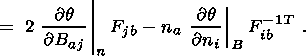
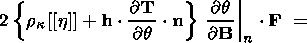
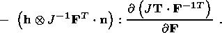
The equation determining the phase transformation temperature as a function of the extension of the initial phase has the form

(4.12)

where L = T/ B is the fourth-rank tensor of elastic moduli.

Equation (4.12) is derived as follows. Using (4.5) and substituting the relation T_k = J T F^-1T between the stress tensors into (4.3), I obtain

The derivative of the phase transition temperature with respect to the tensor F at n_k = const is

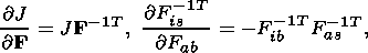
In deriving this equation, I used the formula F^-1T_is/ F_ab = - F^-1T_ib F^-1T_as obtained by differentiating the identity F^-1_si F_ik = d_sk with respect to F_ab. Substituting this expression into the preceding relation gives the equation

Writing out the derivative in the last term, taking into account the formulas

and scalarly multiplying the equation to the right by the tensor F^T, I obtain

Using formula (4.6) and collecting similar terms yield the desired equation (4.12).

In the case of deformed state (4.9) with the shear strain and stress vanishing on the interface, equation (4.12) is reduced to the two simpler relations

(4.13)

(4.14)

where

In order to demonstrate this, I note that formulas (4.10) and (4.11) yield

Since h = [[J]] n for the strain under consideration, I obtain h T n = [[J]] T_nn. Hence, the first term on the right-hand side of (4.12) is equal to [[J (T_ab - d_ab T_nn)]] e_a e_b, and the second term vanishes due to (4.9) and collinearity of the vectors h and n. The last term is equal to

These expressions can be obtained by differentiating polynomial representation (2.7) of the Cauchy stress tensor with due regard for definition (2.8) of the principal invariants I_k ( B), k = 1, 2, 3, and the Hamilton-Cayley theorem [Lurye, 1980]:

Since in the case of deformation (4.9) the value (b₁ + 2 b₂ B₀ + b_IJ B^I+J₀) is equal to T_nn/ B₀, relations (4.13) and (4.14) are proven.

5. Linear, Initially Isotropic Thermoelastic Material

As an example, also interesting on its own, I address the first-order phase transition in an initially isotropic thermoelastic solid with small deformations and small deviations of temperature from its initial value. Let k be the undistorted reference configuration of a material element in the initial phase state. As a reference configuration of this element in the other phase state, the same configuration k, which will also be undistorted due to the isotropy of the medium, is used. The temperature of the material in k is set equal to q₀ and its mass density is denoted as r_k. The initial state of the first phase is regarded as a natural (unstressed) one, and the second phase in the configuration k is characterized by an isotropic initial stress state T₀ = - p₀ I. Deformations of each phase measured from the configuration k and temperature variations are set to be small. A constant singular source of entropy is assumed. The free energy density is smooth in the vicinity of the initial state of each phase and can then be written accurate to second-order terms in the form

(5.1)

where n = 1, 2, is the number of phase; e is the small strain tensor; I₁ = I: e, = q - q₀, /q₀ 1; and the coefficients y⁽ⁿ⁾_k, p⁽ⁿ⁾_k, h⁽ⁿ⁾_k, c⁽ⁿ⁾, a⁽ⁿ⁾, l⁽ⁿ⁾ and m⁽ⁿ⁾ are functions of the temperature q₀. The entropy density and stress tensor in such a material are written in the form of linear relations:

(5.2)

They suggest that l⁽ⁿ⁾ and m⁽ⁿ⁾ are the Lame coefficients, a⁽ⁿ⁾ is the thermal expansion coefficient, c⁽ⁿ⁾ is the heat capacity, and the values y⁽ⁿ⁾_k, h⁽ⁿ⁾_k and p⁽ⁿ⁾_k characterize the free energy, entropy and pressure in the initial states. I assume p⁽²⁾_k = p₀, y⁽²⁾_k = y₀, h⁽²⁾_k = h₀ and p⁽¹⁾_k = y⁽¹⁾_k = h⁽¹⁾_k = 0. Relations (5.2) show that the approximation of small deformations is valid if the initial pressure is small compared to the elastic moduli.

As follows from second relation in (5.2), the jump in the stress tensor at the interface has the form

(5.3)

Using the stress vector continuity condition [[ T]] n = 0, I obtain

(5.4)

where m is the component of the vector e n tangent to the interface.

Now I address relation (3.23) determining the jump in the free energy density; for the subsequent analysis, (3.23) is convenient to use in the form

(5.5)

Taking into account the relations

and formula (5.4), equality is reduced to the form

(5.6)

Taking into account expression (5.4) for the vector h, equation (5.6) implies that, if the dimensionless entropy jump is h = O(1), the phase transition temperature is

i.e. it is only determined by the y and h values and by the dissipation d. The incorporation of terms on the order of O(d²) is unreasonable in the approximation considered, because equations (5.2) are written accurate to the terms of the second order of smallness.

In the case h = O(d) the phase transition temperature appreciably depends on the strain tensor of the initial phase and the orientation of the normal to the interface relative to the principal axes of the tensor e. Before examining this dependence, note that the difference between thermoelastic coefficients of the phases can be, generally speaking, rather large [Babichev et al., 1991]. Therefore, I consider the following case:

In accordance with (5.3) and (5.5), the equation for the phase transition temperature derivative with respect to the vector normal is written in this approximation as

This implies, according to the general theory, that the phase transition temperature at a fixed strain of the initial phase assumes an extreme value if the normal to the interface coincides with a principal axis of the strain tensor,

(5.7)

because m = 0 at such a strain and therefore / n = 0. The type of the extremum is determined by the matrix ² / n n at strain (5.7).

The equation for the phase transition temperature derivative with respect to the strain tensor is written as

(5.8)

Equation (5.8) leads to an important general statement concerning the phase transition pattern in the material considered: an increase in the volume strain changes the type of the phase transformation in a linear thermoelastic solid, i.e. a normal phase transition changes to an anomalous transformation and vice versa. Of course, this refers to materials in which the phase transition is accompanied by a change in the elastic moduli comparable with their values, and the difference between the initial entropies is on the order of h = O(d). The aforementioned effect is solely due to the solid-state properties of the material (the presence of a stress deviator and its effect on the equilibrium state energy of the medium).

Actually, at a fixed normal and a constant intensity of shear strain, I₂ = ( e: e)^1/2 = const, where e = e - ¹/₃ I₁ I is the strain tensor deviator, the phase transition temperature derivative with respect to the first invariant is

The right-hand side of this equation vanishes if the strain tensor component normal to the phase boundary is connected with the two other diagonal components through the relation

Such a strain tensor provides a phase transition temperature extremum with respect to I₁. If the thermal expansion coefficients a = O(d) differ only slightly, this relation can be written, accurate to the first-order terms, in the explicit form

(5.9)

In the case of uniform extension (compression), when the deviator e vanishes, this relation has a particularly simple form:

In the general case, deformations providing an extremum of the phase transition temperature are determined by the solution of the system consisting of equation (5.9) and the condition e: e = const (a constant shear intensity).

6. Effects of Stress Relaxation

Now I analyze, following the work [Kondaurov and Nikitin, 1986], some characteristics of phase transformations accompanied by stress relaxation in the solid phase. The solid phase is described in terms of the model of a viscoelastic medium of the relaxation type. In this case, the state of a material particle is determined by its deformation, temperature, temperature gradient and viscous deformation, and the system of relations governing the material response includes a viscous law in addition to expressions for the thermodynamic potential, stress tensor and heat flux. Below I restrict myself to the simplest case of an initially isotropic viscoelastic material of the solid phase. Moreover, the medium is supposed to be a perfect, plastically incompressible material. Such a model has the following implications. The gradient F of the transformation mapping a neighborhood of a material element X from the initial configuration k into the actual configuration c(t) can be represented as the composition [Kondaurov and Nikitin, 1990; Lee, 1969]

(6.1)

of the gradients of the nondegenerate transformations k k_p ( X, t) and k_p ( X, t) c (t) mapping the reference configuration k into an intermediate (instantly unloaded) configuration k_p ( X, t) which in turn is mapped into c (t). The inelastic volume strain is det F_p = 1. Rheological relations constituting a system of equations of state and kinetic equation of viscous deformations can be written in the form

(6.2)

(6.3)

where y { B_e, q} and q { B_e, q, q} are isotropic functions of the free energy and heat flux vector;

(6.4)

is the symmetrical tensor of viscous strain rate, B_e = V²_e is the symmetrical, positively definite tensor of elastic strain; I_k ( B_e), k = 1, 2, 3, are the principal invariants of the tensor B_e;

(6.5)

are the polar decompositions into orthogonal and symmetrical, positively definite tensors, from which the following relations are derived using composition (6.1):

(6.6)

Constitutive equations (6.2)-(6.3) are necessary and sufficient in order that (i) the Clausius-Duhem inequality hold true in all smooth processes of deformation and temperature variation; (ii) the equations be independent of the choice of the reference system; (iii) the equations be invariant under orthogonal transformations of the unloaded configuration k_p ( X, t) of an infinitely small material element X; (iv) the equations be invariant under arbitrary unimodular transformations of the initial configuration.

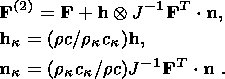
Since U_p is a symmetrical, positively definite tensor, relations (6.3)-(6.4) can be resolved with respect to U_p. This means that the flow law can be written in the form

(6.7)

Relation (6.7) is the divergent equation describing the elastic strain variation rate in the Lagrangian (material) variables X. The divergent form of equation (6.7) in the Eulerian (spatial) variables is

(6.8)

This equation is readily obtained by adding relation (6.7) multiplied by mass density r and continuity equation (2.10) multiplied by the tensor U_p. Relation (6.7) or (6.8) implies that

(6.9)

at the interface, which is a strong discontinuity surface; here w is the intensity of a singular source of inelastic deformations on the interface. This value determines the jump in the viscous strain of a material particle crossing the interface and is one of the factors controlling the stress drop associated with the formation of a new phase and the value of the singular dissipation source in equation (3.12). The value w is one of rheological characteristics that are preset in the model of the quasi-static phase transition in solids.

To illustrate the properties inherent in phase transformations during stress relaxation in the solid phase, I consider the problem of melting of a viscoelastic solid layer. Let an unstressed layer of a constant thickness b occupy the region 0 x b in the initial state (the axis x = x¹ is perpendicular to the layer boundaries, and the axes x² and x³ lie in the boundary plane x¹ = 0 ). The temperature of the material q₀ is below the melting temperature in the absence of stresses. The boundary x = 0 is fixed and its temperature is maintained constant and equal to q₀ at t0. A constant normal compressive stress - s₀, s>0, is applied to the boundary x = b at the time t = 0, and the temperature of the medium increases to a value q₁ = const>0 at which a part of the layer adjacent to the boundary x = b melts. The boundary of the melting region is found from the solution of the problem. Mass forces and distributed heat sources are neglected.

The temperature distribution in the solid phase and melt is assumed to be linear across the layer:

This assumption implies that the heat conductivity of the material is so high that the characteristic time of the temperature buildup is negligibly small compared to the stress relaxation time.

I assume that deformations due to compression, heating and melting are small. The solid phase is modeled by a homogeneous isotropic perfect viscoelastic material with the density r_s and temperature q₀ in the natural initial state k_s. The free energy density of the solid phase occupying the region 0 x a(t) can be written as

(6.10)

where I₁ = e^(e)_kk and J = e^(e)_ij e^(e)_ij are the first and second invariants of the elastic strain tensor e^(e), = q - q₀, /q₀ 1, is the temperature variation, l (q₀) and m (q₀) are elastic moduli, a_s (q₀) is the coefficient of thermal expansion, and g_s (q₀) is the heat capacity (accurate to the multiplier q₀ ). The difference between the densities in the reference and actual configurations is ignored due to the smallness of deformations. As follows from (6.10), the stress tensor and entropy density in the solid phase have the form

(6.11)

The complete strain tensor e is the sum of the elastic (  e^(e) ) and viscous (  e^(p) ) strain tensors:

(6.12)

where u is the vector of displacement from the initial state to the current state.

The variation rate of the viscous strain e^(p) is determined by viscous flow law (6.3); within the framework of the assumptions adopted, the latter reduces to the relation

(6.13)

where S = T - ¹/₃ ( T: I) I is the stress tensor deviator and t (q₀) > 0 is the relaxation time.

The natural (unstressed) reference configuration k_f of the body in the liquid state with the temperature q₀ is represented by a plane layer of the density r_f. The phase density difference is set to be small: (r_s - r_f)/r_s1. Due to the similarity between r_s and r_f, the melted layer thickness b_f = b (r_s/r_f)^1/3 differs only slightly from b. Using the configuration k_s of the layer in the solid state as a reference configuration with initial stresses for the melt, the free energy density of the liquid occupying the region a (t) x b can be written as

(6.14)

where g_f, a_f and K_f are functions of q₀, and the value I₁ = 1 - r/r_s determines the volume strain in the melt measured from the configuration k_s. The value y is the difference between the phase potentials in the configuration k_s, and T = - p I is the tensor of "initial" stresses in the melt occupying the region k_s. If the initial density of the solid phase exceeds the melt density ( r_s > r_f), we have p > 0, i.e. the melt should be compressed in order to make the solid and liquid phase densities equal to each other, and vice versa, p < 0 if r_s < r_f. The dependences of pressure and entropy density on mass density and temperature of the melt as determined by (6.14) have the form

(6.15)

This implies that K_f is the bulk modulus, a_f is the thermal expansion coefficient and g_f is the heat capacity of the liquid phase (accurate to the multiplier q₀ ).

Let u(x, t) be the material particle displacement along the x axis. All other components of the displacement vector in both phases are set equal to zero. Then, the nonzero component of the complete strain tensor is

The equilibrium equation p/ x = 0 and the boundary condition p (b, t) = s₀ yield

Substituting this expression into the first formula in (6.15) and integrating in x, I obtain

(6.16)

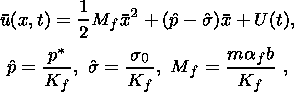(6.17)

where x = x/b and u = u/b are the dimensionless coordinate and displacement, and U (t) is an unknown function of time determined from the solution of the problem. The free energy density of the melt is then reduced to the form

(6.18)

Now I consider the equations for the solid phase under conditions of the uniaxial strain

where e₁ is the basis vector of the Cartesian coordinates xⁱ. Taking into account the symmetry of the problem about the x axis and the zero value of the inelastic volume strain, the viscous strain tensor can be written as

and the elastic strain tensor, as

this yields I₁ = u and J = (u - 2p)² + 2p². Given a uniaxial strain, free energy density (6.10) reduces to the form

(6.19)

The stress tensor at a uniaxial strain is T = s₁₁ e₁ e₁ + s₂₂( e₂ e₂ + e₃ e₃), and the system of equilibrium equations is reduced to the single equation

Hence, the normal stress s₁₁ in the solid phase is constant:

In the uniaxial strain case, the first formula in (6.11) relating the elastic strain and temperature to the stress tensor yields

(6.20)

The evolutionary equation of plastic strain (6.13) in the uniaxial case has the form

and its general solution is

(6.21)

where f(x) is an unknown function of the spatial coordinate x to be determined.

In order to find f(x), note that "instantaneous" (over a time t t ) melting of the part of the layer in the region a(0) x b takes place as soon as the temperature at the boundary x = b increases to the value = ₁ > ₀ at the time t = 0, and the stress becomes equal to s₁₁ = - s₀. The solid phase occupying the region a(0) x b at this time moment remains in the elastic state because the viscous strain does not change over this time interval. Further development of the process is controlled by the accumulation of viscous strain and can be accompanied by an interface motion due to the effect of the viscous strain on the stress state and energy of the solid phase. Therefore, the function f(x) is determined from the condition that the viscous strain vanishes at t = 0. Using (6.21), I find

The expression for the plastic strain can then be written as

(6.22)

Relation (6.22) specifies, in a comprehensive manner, the viscous strain field, provided that the region occupied by the melt monotonically increases with time due to the stress relaxation, i.e. a (t) a (0), a (t) 0. Then, the solid phase region 0 x a (t) decreases with the time t, and the solution is completely determined by the initial data specified at t = 0 in the interval 0 x a (0). In this case, formulas (6.20) and (6.22) yield

(6.23)

Hence, using the boundary condition u(0, t) = 0, I obtain the expression for the displacement

(6.24)

The unknown function U(t) in (6.17) and the dimensionless coordinate of the phase boundary Z(t) = a(t)/b are determined by the coupling conditions at the interface. These are continuity conditions for the normal component of chemical potential (3.23) and displacement (3.2):

(6.25)

It is supposed here that the dissipation vanishes, d = 0. The continuity condition for the temperature and stress s₁₁ holds identically, and condition (6.9) for inelastic deformations is not used because the new phase is an ideal liquid.

Using (6.16), (6.18), (6.19), (6.23) and (6.24), coupling conditions (6.25) are written in the form

(6.26)

where

In what follows, I assume for simplicity that the differences of the bulk modulus, thermal expansion coefficient and heat capacity in the solid phase differ only slightly from the respective values in the liquid phase, i.e.

where |d| 1 is a small parameter characterizing the strain value of the material. Let the rheological characteristics of the phase transition be y = O(d²) and h = O (d²) and let the initial stress in the melt be p = O(d). In this case, the following estimates are valid accurate to the terms O(d²):

At the initial time moment t = 0 the coefficients of system (6.26) are

Substituting the resulting expressions into (6.26) and taking into account definitions (6.18) of the values y and h, the following equation is obtained:

(6.27)

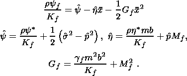
Hence, the melting onset corresponding to Z₀ Z(0) = 1 is controlled by the value M_f = M⁰_f ( s, w, y₀, h₀, p) equal to the minimal positive solution of equation (6.27) and depends on characteristics of the phase transition y₀, h₀ and p, parameter 0 w 1 - K_s/L 1 and applied load s.

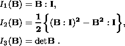
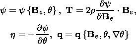
Figure 1

If the temperature gradient is M⁰_f < M_f < , a part of the layer melts. The coordinate 0 < Z₀ < 1 is determined by the expression

where Y is, as before, the minimal positive solution of equation (6.27). The dependence of the initial position of the interface on the stress s applied to the layer is shown in Figure 1 for the values w = 0.1, 0.3, 0.6, 0.75 and 0.9 (respective curves 1-5). Figure 1a shows the dependence Z₀( s) for p = 0.5 s , i.e. for the "normal" phase transition, with the density of the solid phase exceeding the melt density. The value s is a characteristic stress such that s/L = O(d). Figure 1b shows similar curves, with the same values of w, for p = - 0.5 s ("anomalous" phase transition).

A characteristic feature of these curves is a monotonic variation (a decrease or increase in the respective cases of normal or anomalous transition) in the initial thickness of the melt layer 1 - Z₀ with increasing compressive s at small w (curves 1 and 2 in Figure 1a). The behavior of curves 1 and 2 is consistent with traditional notions of the classical theory of phase transitions: the applied pressure increases the temperature during the normal phase transition and decreases it during the anomalous one. However, as w increases, the dependence of the initial melt thickness on the applied pressure becomes nonmonotonic. The function Z₀( s) (curves 3-5) has a maximum that shifts, with increasing w, toward smaller applied pressures for both normal and anomalous phase transitions. This feature is related to the effect of solid-state properties on the phase transformation pattern noted in section 5. In the vicinity of stress states, where d Z₀/d s , this can lead to instability of the phase boundary and, in particular, to dynamic phenomena with slowly varying boundary conditions.

Examination of the function Z(t) at t > 0 shows that the derivative d Z(t)/dt is positive at all of the considered values of the phase material parameters, applied load and temperature gradient. This contradicts the initial assumption on sign of the derivative Z(t).

The problem considered excludes the case of a phase boundary retreating after a part of the material had instantly melted ( Z(t) > Z(0) ). Actually, suppose that Z(t) > 0. Then the viscous strain of a solid phase particle forming from the melt at the interface vanishes. Using the first coupling condition in (6.25) at the interface (the continuity of the normal component of the chemical potential tensor) and taking into account formulas (6.16) and (6.18)-(6.20), it is readily seen that this equation gives a constant value of the interface coordinate, because the values in the relations considered are time independent. Consequently, a retreating motion of the phase boundary is impossible in the problem with boundary conditions considered. This means that the melt boundary coordinate remains constant at t > 0, and the surface x = Z(0) is a contact discontinuity. In accordance with (6.22) and (6.23), the total and viscous strains change in solid phase material particles adjacent to this surface. Since the viscous strain vanishes in a melt particle at the contact boundary, the following relation holds:

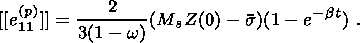The evolution of the viscous strain at the contact discontinuity under consideration leads at t > 0 to a jump in the normal component of the chemical potential:

In accordance with (6.26), the value of this jump can be written as

To sum up, the following features of phase transitions in solids associated with the presence of stress relaxation are noteworthy.

An abrupt change in the boundary conditions that occurs over a time small compared to the characteristic time of stress relaxation is accompanied by a rapid movement of the phase boundary and complies with an instantaneous elastic response of the material.

The evolution of plastic deformations at constant boundary conditions can either increase or decrease the volume of the new phase, i.e. the interface can retreat [Kondaurov and Nikitin, 1986]. The interface motion pattern depends on the geometry of the region, boundary conditions and material parameters.

As the boundary conditions attain a stationary regime, the phase boundary can be transformed into a contact discontinuity immobile relative to material particles. Jumps in the tangential component of the displacement vector, viscous strain and normal component of the chemical potential can arise at this discontinuity surface.

Solid-state properties of the material can result in unstable behavior of the phase boundary, including dynamic phenomena at slowly varying boundary conditions.

References

Babichev, A. P., N. A. Babushkina, A. M. Bratkovskii, et al., A Handbook of Physical Quantities (in Russian), Energoatomizdat, Moscow, 1991.

Bowen, R. M., Toward thermodynamics and mechanics of mixtures, Arch. Rat. Mech. Anal., 24, (4), 370-403, 1967.

Bushman, A. V., I. V. Lomonosov, and V. E. Fortov, Equations of State of Metals at High Energy Densities (in Russian), IKhFCh RAN, Chernogolovka, 1992.

Christian, J., Theory of Transformations in Metals and Alloys (in Russian), vol. 1, Mir, Moscow, 1978.

Coe, R. S., The thermodynamic effect of shear stress on the orthoclinoinversion in enstatite and other coherent phase transition, characterized by finite simple shear, Contribs. Mineral and Petrol., 26, 247, 1970.

Gibbs, J. W., The scientific papers, Thermodynamics, vol. 1, Longmans, Green and Co, New York, 1906.

Grinfeld, M. A., Methods of Continuum Mechanics in the Theory of Phase Transformations (in Russian), Nauka, Moscow, 1990.

Khachaturyan, A. G., Theory of Phase Transformations and the Structure of Solid Solutions (in Russian), Nauka, Moscow, 1974.

Knyazeva, A. G., Generalizations of the Clapeyron-Clausius equation in a self-consistent thermomechanical model (in Russian), PMTF, 40, (6), 103-111, 1999.

Kondaurov, V. I., On conservation laws and symmetrization of nonlinear thermoelastic equations (in Russian), DAN SSSR, 256, (4), 819-823, 1981.

Kondaurov, V. I., and L. V. Nikitin, Study of first-order phase transitions in nonlinear elastic media (in Russian), Izv. AN SSSR, MTT, (6), 49-55, 1983.

Kondaurov, V. I., and L. V. Nikitin, First-order phase transitions in an elastic- viscoplastic Medium (in Russian), Izv. AN SSSR, MTT, (4), 130-139, 1986.

Kondaurov, V. I., and L. V. Nikitin, Theoretical Foundations of Rheology of Geomaterials (in Russian), Nauka, Moscow, 1990.

Kulikovskii, A. G., and E. I. Sveshnikova, Nonlinear Waves in Inelastic Media (in Russian), Nauka, Moscow, 1998.

Landau, L. D., and E. M. Lifshits, Statistical Physics (in Russian), Nauka, Moscow, 1964.

Landau, L. D., and E. M. Lifshits, Hydrodynamics (in Russian), Nauka, Moscow, 1988.

Lee, E. H., Elastic-plastic deformation at finite strain, Trans. ASME. J. Appl. Mech., 36, (1), 1-6, 1969.

Lurye, A. I., Nonlinear Theory of Elasticity (in Russian), Nauka, Moscow, 1980.

Mukhamediev, Sh. A., Fracture Processes in the Earth's Lithosphere (in Russian), IFZ RAN, Moscow, 1990.

Melosh, H. G., Impact Cratering: A Geological Process, Oxford Univ. Press, New York, 1989.

Ostapenko, G. T., Thermodynamics of Nonhydrostatic Systems and its Applications in the Theory of Metamorphism (in Russian), Naukova dumka, Kiev, 1977.

Ovsyannikov, L. V., Lectures on Fundamentals of Gas Dynamics (in Russian), Nauka, Moscow, 1981.

Robin, P. Y. F., Thermodynamic equilibrium across a coherent interface in a stressed crystal, Amer. Miner., 59, (11-12), 1286, 1974.

Roitburd, A. L., Theory of the heterogeneous structure formation due to phase transformations in solids (in Russian), UFN, 113, (1), 69-104, 1974.

Rozhdestvenskii, B. L., and N. N. Yanenko, Systems of Quasi-Linear Equations and Their Applications in Gas Dynamics (in Russian), Nauka, Moscow, 1978.

Sadovskii, V. M., Discontinuous Solutions in Dynamic Problems of Elastic-Plastic Media (in Russian), Nauka, Moscow, 1997.

Sedov, L. I., Continuum Mechanics (in Russian), vols. 1 and 2, Nauka, Moscow, 1970.

Truesdell, C., A First Course in Rational Continuum Mechanics, Johns Hopkins Univ., Baltimore, Maryland, 1972.

Truskinovskii, L. M., On the chemical potential tensor (in Russian), Geokhimiya, (12), 1730-1744, 1983.

Turcott, D. L. and G. Schubert, Geodynamics: Applications of Continuum Physics to Geological Problems, John Wiley, New York, 1982.