
Electromagnetic phenomena preceding and accompanying seismic events continue to attract attention not only as possible earthquake precursors but also as additional parameters for describing the earth’s crust and its dynamics. Before considering seismo-electromagnetic (SEM) phenomena, however, we address the question of whether such phenomena do in fact exist.
In spite of the publication of several hundred articles from the beginning of the twentieth century dealing with the relationship between EM signals and pre-seismic processes in the earth’s crust, there is still no definitive proof that the two are connected. While there are several reasons for this, we think that the main reason is the practical impossibility of repeating the results of field observations. It is necessary to wait a long time, sometimes many years, for a large earthquake to occur with similar parameters in approximately the same location.
A second reason is that areas of high seismic activity usually differ widely in geological and seismic characteristics. In addition such areas generally have a high degree of geological inhomogeneity. Both of these factors make the planning of field experiments and the interpretation and comparison of results difficult.
Thirdly, to capture an SEM signal, one must distinguish it from the background, which consists of both natural and man-made EM noise spanning a broad frequency range.
Finally, various research groups have used different measurements and discrimination techniques and frequency ranges, which limits comparison of their results.
Taken together, the above factors have contributed to a lack of consensus among the many research groups which have investigated the existence of SEM phenomena over the past century. Nevertheless we list here some evidence for a positive answer to the question posed in the opening paragraph.
1. The phenomenon of mechano-electromagnetic transduction has been well studied in the laboratory in a wide variety of solids including rocks [Cress et al., 1987; Kapitsa, 1955; Khatiashvili, 1984; Nitsan, 1977; Ogawa et al., 1985; Parkhomenko, 1971; Schloessin, 1985; Volarovich and Parkhomenko, 1955; Volarovich et al., 1962; Yamada et al., 1989].
2. Creation of an electric field by the passage of a seismic wave through soil has been observed [Eleman, 1965; Ivanov, 1939; Leland and Rivers, 1975; Martner and Sparks, 1959]. These seismo-electric effects have been applied to geophysical prospecting [Kepis et al., 1995; Sobolev and Demin, 1980; Sobolev et al., 1984; Thompson and Gist, 1993].
3. The emission of EM signals has been observed in the field experiments over distances as small as tens to hundreds of meters [Mastov et al., 1983, 1984; Solomatin et al., 1983a, 1983b]:
4. The unusual appearance of local atmospheric light seconds or minutes before, and close to the epicenter of, some earthquakes has been witnessed by many individuals [Derr, 1973; Ulomov, 1971; Yusui, 1968]. Obviously, the appearance of atmospheric light implies the existence of strong electric fields.
5. Some pre-seismic data show unusual EM signals. For example, Fraser-Smith et al. [1990] monitored EM signals 7 km from the epicenter of the strong Loma Prieta earthquake of 1989. Starting forty days before the quake and continuing for several weeks after the quake, anomalous signals were detected. In particular, three hours before the quake, disturbances began which exceeded the background noise by two orders of magnitude.
The above reasons provide a basis for serious consideration of the existence of SEM phenomena. Such phenomena have been discussed in several monographs and reviews [Gokhberg et al., 1995; Hayakawa and Fujinawa, 1994; Johnston, 1989, 1997; Lighthill, 1996; Park, 1996; Park et al., 1993; Rikitake, 1976a, 1976b]. We wish to describe briefly a scenario for them based on 1) analysis of experimental field and laboratory data and 2) modeling of electromagnetic emission which incorporates a mechanical model for pre-seismic deformation developed by us over the past fifteen years [Dobrovolsky et al., 1989; Gershenzon, 1992; Gershenzon and Gokhberg, 1989, 1992, 1993, 1994; Gershenzon et al., 1986, 1987, 1989a, 1989b, 1990, 1993, 1994; Grigoryev et al., 1989; Wolfe et al., 1996]. We have used specific mechanical models of pre-earthquake processes [Dobrovolsky, 1991; Karakin, 1986; Karakin and Lobkovsky, 1985] in some of these articles. But we will not use any of them in this paper because no one model is good enough to describe such complicated processes and developing such a model is not a goal of this paper. Furthermore a specific mechanical model of pre-seismic processes is not needed in constructing a model for SEMS.
The final stage of an earthquake cycle is characterized by stress release processes including foreshocks, the main shock (or swarm), aftershocks, and creep (before and after the earthquake). All of these processes are accompanied by formation of a number of cracks since the Earth's crust consists of extremely brittle materials. So we suppose that the initial source of most SEM anomalies is a localized high density of cracks. Such questions as how these localized regions of high crack density are related to the earthquakes, and how far from the earthquake origin and how long before the earthquake they appear, are not considered here. Part of the mechanical energy released in the formation of these cracks is transformed into electromagnetic energy by a variety of mechanisms. Typical "transducer'' mechanisms in crustal rocks include piezomagnetic, classical and non-classical piezoelectric, electrokinetic and induction. Under appropriate but realistic conditions, phenomena such as quasi-static geomagnetic and electrotelluric anomalies, ultra-low-frequency (ULF) magnetic variations, and radio-frequency (RF) emissions, all associated with pre-seismic processes, can be explained and estimated on the basis of known mechanical and electromagnetic parameters of the earth's crust.
A comparison of our estimated values of seismo-electromagnetic signals (SEMS) with reported field measurements leads to the conclusion that the sources of most anomalous SEMS are relatively close to the detector. In other words, the source of the signal is local. We expect that all pre-earthquake processes, including SEMS, are connected indirectly through global shear stresses, in agreement with Kanamori's interpretation of both SEMS and earthquakes as manifestation of regional geophysical processes [Kanamori, 1996].
There is a recognition that clarification of the physical mechanisms of SEMS generation, transmission and reception is needed [Uyeda, 1996]. We address these problems in the sections that follow. In section 2 the spectral density of a mechanical disturbance associated with the appearance of a crack is introduced. Section 3 will describe the various coupling mechanisms between a mechanical disturbance and the resulting electromagnetic disturbance. Formulas will be given which relate the parameters of the mechanical disturbance to the parameters which produce the EM disturbance (e.g. magnetization, polarization, current density). This section also includes a comparison of the strengths of these EM sources. Section 4 connects, via Maxwell's equation, the resulting SEMS to the electrical and mechanical parameters of the crust and the characteristics of the mechanical disturbance. The formulas enable us to estimate the spectral density of the SEMS for each type of source considered here. Section 5 describes briefly the morphological features of several observed SEM phenomena, namely tectonomagnetic variation, electrotelluric anomalies, geomagnetic variation in the ultra-low frequency range, and electromagnetic emission in the RF range. The interpretation of these phenomena is discussed based on our model. The paper concludes with a summary of our results and suggestions for future field experiments.
It is natural to suppose that the origin of SEM anomalies lies in mechanical processes occurring in the earth's crust before an earthquake. The large build-up of mechanical energy during deformation is expended mainly through stress relaxation before, during and after the quake, but a small part goes into EM emission. Note that an important circumstance is that the vibrational spectrum associated with the release of mechanical energy, since it arises, on an atomic scale, from the motion of atoms carrying an electrical charge or a magnetic moment, is related to the spectrum of the EM emission. So if we observe an SEM anomaly of a certain frequency, there must be an associated mechanical disturbance of the same frequency. This does not imply that the corresponding spectral densities are identical, because the electro-mechanical coupling is frequency-dependent. But we would not expect a large EM emission peak in a frequency range where the vibrational spectral density is very small.
|
|
| Figure 1 |
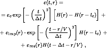
In this figure, the crack begins to grow at t=0. As it opens, a strain pulse propagates away from the crack, reaching point xi at time ti ( i = 1, 2, 3). The pulse grows to a maximum value and, after it passes, the strain relaxes to a steady value. The maximum and steady values fall off with distance from the crack, but the duration of the pulse, Dt, is constant and given by lc/Vc where lc is the crack size and Vc is the crack opening speed (speed of propagation of the crack tip). The quantity Vc is a complicated function of the type of crack, the elastic modulus of the material and the details of the crack formation process, but is less than the velocity of Rayleigh wave [Kostrov, 1975] and independent of crack size, having a characteristic value of order 1 km/sec [Kuksenko et al., 1982].
From Figure 1b, we see that the appearance of a crack gives rise to a seismic impulse. The magnitude of this strain impulse is large near the crack and there remains a residual value at long times. We want to estimate the spectral density of mechanical vibrations associated with this impulse. Assume that the change in strain varies with time according to
 | (1) |
where H(r) is the unit step function ( H(r) is zero for r<0 and one for r>0 ), r is the distance from the crack, V is the elastic wave velocity, ec is the average strain change in the vicinity of the crack, e imp(r) is the strain change due to the seismic impulse, and e res(r) is the change in residual strain due to formation of the crack.
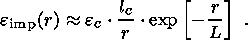
The quantity e imp(r) decreases with r as r-1 as the pulse propagates away from the crack. But it also is attenuated by the factor exp[-r/L] due to inelastic processes, where L is the attenuation length. We represent e imp(r) as
 | (1a) |
The attenuation length is a complicated function of frequency, rock structure, temperature and pressure, and can range from 10 to 10,000 wavelengths [Carmichael, 1989]. In this paper we shall assume that L lies in the range 10lc to 103lc. The strain e res(r) falls off with distance much more quickly than e imp(r). We assume
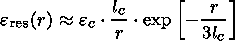 | (1b) |
which expresses the fact that the residual strain extends to about three time the crack size.
Now we can find the spectral density for e(t, r) using equations 1, 1a, and 1b. The result is
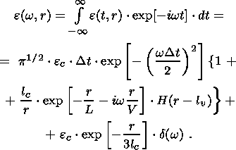 |
The spectrum includes a zero-frequency spike (last term on the right) and a broad,
flat spectrum from
w=0 up to the frequency
wc=(Dt)-1.
As we will see in Section 4, the existence of a characteristic pulse lifetime
t=L/V adds a narrow, flat portion
from
w=0 up to
w imp=(t)-1.
For
L=102lc, V=3Vc,
and
lc=1 mm,
10-1 m and 10 m, the value of
wc is of order 10
6, 104, and
102 rad/s, respectively, and that
of
w imp is
3 104, 300 and 3 rad/s. A result
analogous to the
preceding expression is obtained for the change in volume strain,
q(w, r).
104, 300 and 3 rad/s. A result
analogous to the
preceding expression is obtained for the change in volume strain,
q(w, r).
Under natural conditions, practically all rocks contain pore water. In Section 5 we will show that the diffusion of pore water plays a major role in some SEM phenomena.
As shown in equations A6 and A9 of Appendix A, when monochromatic elastic waves propagate through the crust, the pressure change P is proportional to the volume strain q for both high and low frequencies. Thus there is a linear coupling between pore pressure and volume fluctuations during a seismic disturbance. This provides us with a means of estimating the relative contribution of pore water diffusion to SEM signals. In particular it enables us to connect changes in crustal deformation and pore water pressure.
Equations A6 and A9 are strictly true only for a monochromatic disturbance. Let's consider again the stress pulse associated with a crack (Figure 1b). While the pulse is growing, the relation between each elastic wave component and the corresponding pore pressure wave component will be given by equation A6 for high frequencies and equation A9 for low frequencies. After the pulse passes, leaving a constant residual stress, the pore pressure will relax according to the diffusion equation A7, as in Figure 1c.
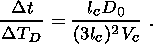
In this figure, the pore pressure has a characteristic diffusion relaxation time DTD (see equation A7) given by
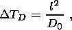 | (2) |
where
l is the linear extent of the region in the vicinity of the crack which has
appreciable residual
stress
(l 3lc), and
D0=K2k0/mvb
3lc), and
D0=K2k0/mvb is the diffusion
coefficient. The quantities appearing in
D0 are defined in Appendix A.
To estimate the frequency spectrum associated with the pressure change
P(t, r) we use an expression similar to equation 1:
is the diffusion
coefficient. The quantities appearing in
D0 are defined in Appendix A.
To estimate the frequency spectrum associated with the pressure change
P(t, r) we use an expression similar to equation 1:
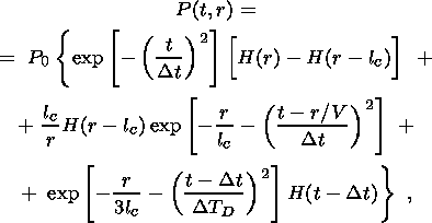 | (3) |
where P0 is the pore water pressure change due to a change of volume strain. We obtain
 |
From this result we see that the spectrum consists of three parts, a broad low-intensity region (first term) and two low-frequency regions of much higher intensity, one related to the seismic impulse (second term) and the other to a pore water diffusion process (third term). The ratio of the intensities in the first and third regions is Dt/DTD. Recall that Dt is given by lc/Vc. Together with equation 2 this gives
 |
Usually this ratio is much less than one, which means that the process related to water diffusion will dominate in the low frequency range.
From the last two subsections we arrive at the following conclusions. Cracks are a source of two types of mechanical disturbances, a seismic impulse and, in the presence of water-saturated rock, diffusion of pore water. The frequency spectrum of these mechanical disturbances in general will consist of four parts. First there is a zero-frequency spike arising from the residual strain. This spike could potentially be a source of tectonomagnetic anomalies (see Section 5). Second there is a broad spectral range from zero up to high radio frequencies, related to the crack-opening process. The spectral density is nearly flat in this range. Third there is a much narrow spectral range from zero up to low radio frequencies, associated with the seismic impulse generated by the crack. Fourth, there is a low-frequency contribution arising from the diffusion of pore water. This diffusion is driven by the stress associated with crack formation through equation A7. The spectral density of this part of the spectrum exceeds by several orders of magnitude the broad flat part.
In our model, the basic source of the SEM anomaly is a mechanical deformation resulting in the formation of a large number of cracks. The volume density of cracks, n, cannot exceed the value n max, which, in agreement with laboratory data [Zhurkov et al., 1977], is related to the typical crack length, lc, via
 | (4) |
If n reaches the value n max, the laboratory sample disintegrates. This implies that n will not exceed n max in the earth's crust. (Some early estimates of the magnitude of SEM anomalies did not take this restriction on n into account [Warwick et al., 1982].) We therefore express the crack density by the relation
 | (5) |
where a is the ratio of the actual to the maximum crack density ( 0<a<1 ).
In general, the growth direction of a microcrack is random. But formation of these cracks is a stress-release mechanism, so we would expect that locally there would be some preferred growth direction. Then the average growth direction in a macro-volume undergoing mechanical deformation would be non-zero. In this case the average volume strain, q, and average shear strain, e, are
 |
where q and e are the typical volume and shear strains near a crack.
Formulas (1, 3, 4, 5, and 5a) will be the basis for calculating the magnitude of the various types of SEM anomaly (see sections 4 and 5).
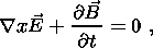
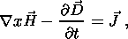
In this section we estimate the contribution of possible sources to the EM field. We start by writing Maxwell's equation (in SI units) for an isotropic medium described by electrical permittivity e, magnetic permeability m and electrical conductivity s:
 | (6a) |
 | (6b) |
 | (6c) |
 | (6d) |
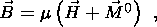
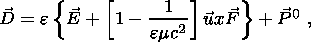
with constitutive relations
 | (7a) |
 | (7b) |
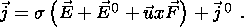 | (7c) |
Here c is the speed of light, u is the velocity of the medium, F is the main geomagnetic field, and j0, E0, P0 and M0 are the external current density, electric field, polarization and magnetization, respectively.
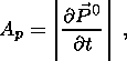
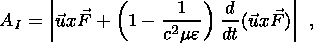
In general we can classify possible sources into three groups: active, passive and apparent. Examples of active sources are
u x F arising from motion of the medium in the geomagnetic field F
By passive sources we mean changes in the electromagnetic parameters s, m and e of the earth's crust due to mechanical processes. An example of a passive source is a change in s in the presence of an external electric field. Such external fields nearly always exist due to magnetospheric/ionospheric geomagnetic variation. Estimation of the effect of passive sources indicates that it is generally much smaller than that of active sources. Therefore we will not consider such sources here, although under special circumstances (e.g. the geometry of local conductivity changes) they may produce anomalies of substantial magnitude [Honkura and Kubo, 1986; Merzer and Klemperer, 1997; Rikitake, 1976a, 1976b].
An example of an apparent source would be the apparent electrotelluric field arising from a change, for whatever reason, of the chemical composition of pore water during measurement of the field, since such a measurement is done using electrodes placed just below the surface [Miyakoshi, 1986]. Another example is a change in the apparent local orientation of a detector due to local displacement of the crust. This would give rise to an apparent change in the EM field in the radio frequency range. Sometimes the amount of local displacement needed to give an observed effect is very small. The existence of apparent sources depends on the type of detector and how it is installed, so it is difficult to discuss them in general. However one should keep their existence in mind when interpreting electromagnetic anomalies.
We want to compare the contribution of different active sources. For ease of calculation we assume that the crust is homogeneous and static, i.e. s, e and m are constants independent of location and time. This makes the use of equations 6 (a-d) and 7 (a-c) convenient. We can eliminate H, B and D and obtain a single equation for the electric field E in terms of its sources:
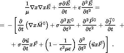 | (8) |
The right-hand side of this equation contains the sources. M0, P0, j0, E0 and u, which are connected to the mechanical state of the crust through various mechano-electromagnetic coupling mechanisms. In order to estimate and compare the effects of the various sources, we need to write down what these coupling mechanisms are.
Some minerals in the earth's crust show residual magnetism due to ferromagnetic inclusions (e.g. titano-magnetite). This residual magnetism was "frozen in'' at the time of formation by the paleogeomagnetic field. The deformation of this type of rock leads to changes in M0 due to changes in the orientation of the inclusions [Kapitsa, 1955; Kern, 1961; Stacey, 1964; Stacey and Johnston, 1972]. These changes are in general a complicated function of the applied stress, the size of the inclusions and the microstructure of the rock, but the following expression is widely used in calculations [Hao et al., 1982; Zlotnicki and Cornet, 1986]:
 | (9) |
where c|| is the stress sensitivity in the direction parallel to the axial load, sij is the stress tensor, I is the reference magnetization and repeated indexes are summed. In terms of the strain tensor eij and the shear modulus ms, we can write
 | (10) |
One of the most commonly occurring minerals, quartz, shows this effect, namely, the occurrence of an electric polarization under the influence of mechanical stress [Parkhomenko, 1971; Volarovich and Parkhomenko, 1955]. Usually, quartz grains are randomly oriented and show very weak piezoelectricity in the aggregate. But because of residual orientation of the quartz grains some rocks will show a larger piezoelectric effect [Ghomshei and Templeton, 1989], although still perhaps two to three orders of magnitude less than in monocrystalline quartz [Bishop, 1981]. The piezoelectric properties of rocks have been widely studied in the context of geophysical prospecting [Kepis et al., 1995; Neyshtadt et al., 1972; Sobolev and Demin, 1980; Sobolev et al., 1984]. Changes in polarization can be related to the strain tensor via
 | (11) |
where
Dkij is the piezoelectric modulus. For
making estimates, we consider only the contribution
from
i=j=1. The magnitude of
Dkij depends on the scale of the mechanical
disturbance. If this scale is of the order of the diameter of a typical quartz
grain (~0.5 mm) then
D Dk11 - 2.3
 10-12
C/N;
if the scale is much larger than this we will take
D -10-14 C/N
[Bishop, 1981].
10-12
C/N;
if the scale is much larger than this we will take
D -10-14 C/N
[Bishop, 1981].
It is possible for the polarization to change for reasons other than the classical piezoelectric effect. All real crystals contain extended defects (dislocations). In dielectric materials, dislocations usually are charged because point defects are associated with them. Under static conditions the charge around the dislocation is neutralized by point defects of opposite charge (the Debye-Huckel cloud). Under the influence of an applied stress the dislocation can move. At nearly all temperatures of interest an unpinned dislocation will move much more quickly than its associated Debye-Huckel cloud and therefore will carry a net charge along with it. This will give rise to charge transport and polarization of the material. This effect was discovered by Stepanov [Stepanov, 1933]. Its magnitude is a complicated function of dislocation density, density and type of point defects, temperature and pressure. Because rocks have an extremely high density of dislocations and point defects, pinning effects will make dislocation movement almost impossible at normal temperatures in these materials; at greater depths where the temperature and pressure are greater this effect could be important [Slifkin, 1996]. There are some mechanisms related to movement or polarization of point defects which also lead to the appearance of an electric field. One of these effect is the so called "pressure stimulated current'' [Varotsos and Alexopoulos, 1986]. Another mechanism for polarization of the crust is directly associated with crack formation [Cress et al., 1987; Khatiashvili, 1984; Nitsan, 1977; Ogawa et al., 1985; Schloessin, 1985; Warwick et al., 1982; Yamada et al., 1989]. It is well known that the appearance of a crack in almost any material produces effects such as light bursts, electron streams and broad-band electromagnetic emission up to x -ray frequencies [Deryagin et al., 1973; Finkel et al., 1985; Gershenzon et al., 1986]. These phenomena are due to the electric field (up to 108 V/m) associated with a buildup of high electric charge density on the new surfaces of the emerging crack. This effect has been studied by several groups and is another type of non-classical piezoelectric effect. It is almost impossible to estimate theoretically the contribution from this mechanism since there are many different effects which accompany crack formation and many unknown parameters, but it could be important in high-frequency SEM phenomena.
As mentioned above, under natural conditions rocks practically always contain pore water. At the pore boundary there exists an electric double layer due to the difference in the electrochemical potentials of water and rock. Deformation of the earth's crust leads to changes in pore pressure and, as a consequence, diffusion of the pore water in a direction opposite the pressure gradient. The motion of this water layer next to the pore boundary results in charge transport, i.e. an electric current, parallel to the boundary. This phenomenon was discovered in the mid-nineteenth century and was first used in a geophysical context by Frenkel [1944] to explain the observations of Ivanov [1939]. More recently it has been used in explaining and modeling SEM phenomena [Ishido and Mizutani, 1981; Mizutani and Ishido, 1976; Mizutani et al., 1976] and in geophysical prospecting [Maxwell et al., 1992; Sobolev and Demin, 1980; Thompson and Gist, 1993; Wolfe et al., 1996]. The relation between the electrokinetic current density j0 and pore pressure P can be written as
 | (12) |
where C is the coefficient of the streaming potential. The pressure is related to the volume strain by equation A1 (Appendix A).
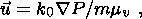
Movement of conducting crustal material in the geomagnetic field gives rise to an induced electric field u x F and current j=su x F. There are two possible sources of this movement; one is the deformation and movement of rock material itself and the other is diffusion of pore water due to volume deformation. In the first case the velocity u of the crustal material is related to the strain tensor eij by
 | (13) |
where V is the velocity of elastic waves. This formula reflects the fact that any change in strain is propagated through the crust at the seismic velocity.
In the case of induction due to pore water movement the effective velocity u can be estimated by Darcy's law,
 | (14) |
where P is given in equation A9 and the parameters k0, m and mv are defined in Appendix A.
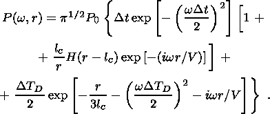
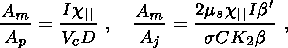
Now that we have expressed all the terms on the right-hand side of equation 8 in terms of electromechanical coefficients and strain changes, we can compare different kinds of sources. Let's consider the terms
 | (15a) |
 | (15b) |
 | (15c) |
 | (15d) |
which are piezomagnetic, piezoelectric, electrokinetic and induction sources,
respectively. We have two
types of induction sources, a source A
I1 due to deformation and movement of rock material
itself and a
source A
I2 due to diffusion of pore water. It is easy to
show that the second term in relation 15d is small
compared with the first term, and we shall neglect it. Replacing
 t with
Vclc
and
r with
1lc,
we can find the ratios of the strengths of the various transducer mechanisms using
equations 9 through 14 and A9:
t with
Vclc
and
r with
1lc,
we can find the ratios of the strengths of the various transducer mechanisms using
equations 9 through 14 and A9:
 |
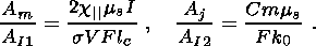 |
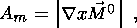
Table 1 shows the results of comparing these strengths for the values of D, C, lc and k0 given in Table 1a. The values of the remaining coefficients appearing in these ratios may be obtained from Table A1 (see Appendix A). We see that the strength of a piezomagnetic source has the same order of magnitude as that of piezoelectric pure quartz. Monocrystalline quartz occurs in nature only as small grains ( < 1 mm), which have practically no preferred orientation ( D=D1 ). For such small grains a piezoelectric source would be important only in the radio-frequency range. If the piezoelectric grains were to have a preferred orientation on a macro-scale ( D=D2 ), we would expect their source strength to be at least two orders of magnitude weaker than a piezomagnetic one.
Referring again to Table 1, comparison of piezomagnetic and electrokinetic sources shows that under some conditions, namely high (but still reasonable) values of electrical conductivity s and electro-streaming potential C, an electrokinetic source could have a strength of the same order of magnitude as a piezomagnetic or piezoelectric source. For low conductivity ( s<10-3/W-m ) the piezomagnetic source exceeds the electrokinetic source.
The three types of sources considered above have the same dependence on the source size; for this reason the latter does not enter into the comparison of their relative strengths. In the case of an induction source of type 1 (AI1 ), the induction source strength relative to the strength of any of the other three sources depends on the size of the source. We can see from Table 1 (first column/fourth row) that the piezomagnetic source essentially exceeds the induction source AI1 on small to medium size scales; the induction source AI1 becomes important only for a source size greater than 1 km and high electrical conductivity ( s>10-1/W-m ).
Both electrokinetic sources and induction sources of the second type (AI2 ) arise from diffusion of
pore water, so they occur together. We see that the induction source AI2 is always much less than the
electrokinetic source. Even if the water layer in the crust has an extremely high
permissibility
( k010-10 m
2 ) the electrokinetic source exceeds AI2 by two to three
orders of magnitude. For usual values of permissibility ( k0 = 10-12 to
10-16 m2 ),
the difference in source strength ranges from four to nine orders of magnitude.
The preceding considerations lead us to the following conclusions. For small sources, the most important mechano-electromagnetic processes considered here are the piezomagnetic, electrokinetic and piezoelectric. For large sources, only piezomagnetic and electrokinetic processes are important. The induction effect is important only on a very large size scale, when the source size is comparable to the earthquake focal zone.
This document was generated by TeXWeb (Win32, v.1.3) on October 28, 2000.